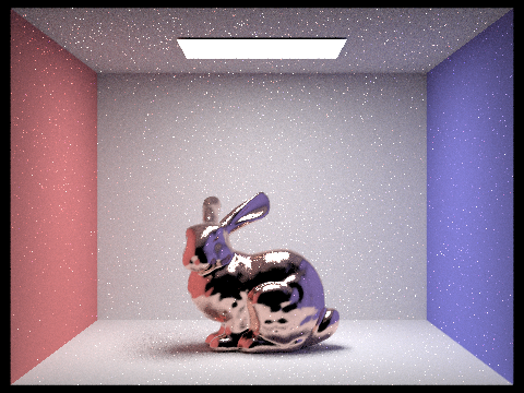
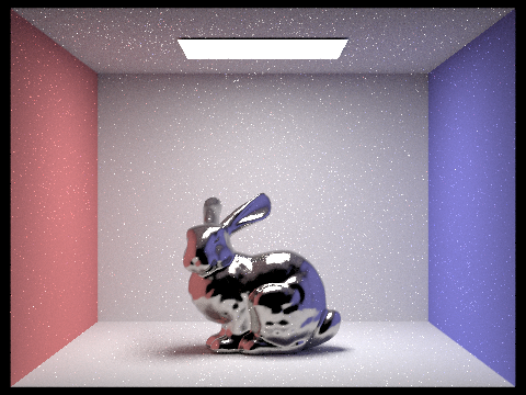
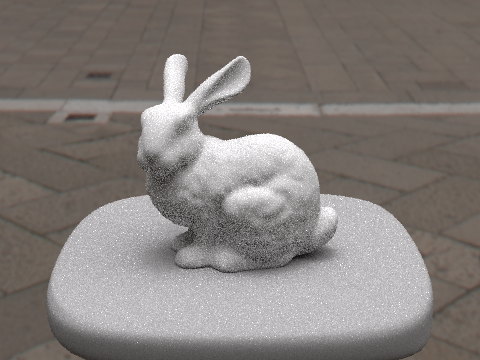
Part 1: Mirror and Glass Materials
Below is a series of renderings of dae/sky/CBspheres.dae at 64 samples per pixel and 4 samples per light.
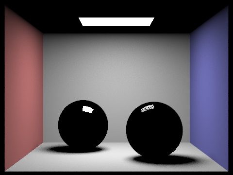
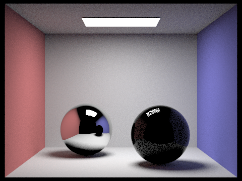
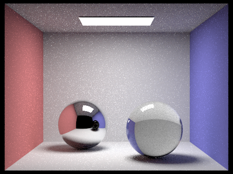
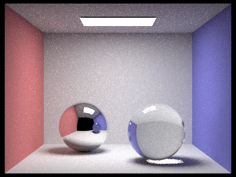
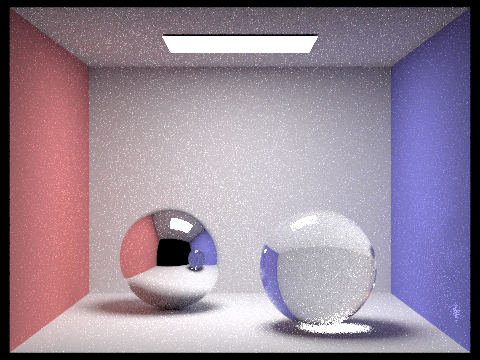
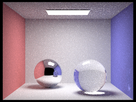
At max ray depth 0, there is no multi bounce effect since only the light directly from the light source is captured. At max ray depth 1, we can see one bounce lights, with the mirror and the glass balls reflecting light off their surfaces from the area light. The scene gets more interesting at max ray depth 2, when the camera rays become reflected to the walls and further to the light source (2 bounces); this gives the mirror ball its shiny look. We can only start to capture the transparency of the glass ball at max ray depth 3 since it takes at least 2 bounces before light could even travel through an object of its material. Here we can see the colors of the walls a lot better than what we could see at max ray depth 2. When we step up to max depth 4, we can see a concentrated area of highlight of the light source passing through the glass sphere. Also there are more colors on the reflected image of the glass ball on the mirror ball. Further, at max depth 5, we could additionally see shiny reflections of light on the wall to the right. There are other areas of highlights as well due to lights rays bouncing within the object. Finally, at max ray depth 100 (most should be terminated a lot earlier by Russian Roulette), we see smoother results of those specular highlights.
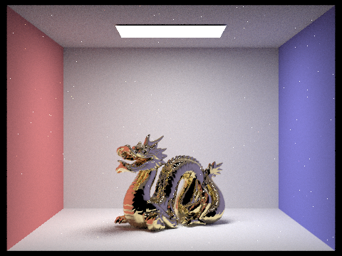
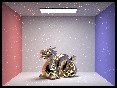
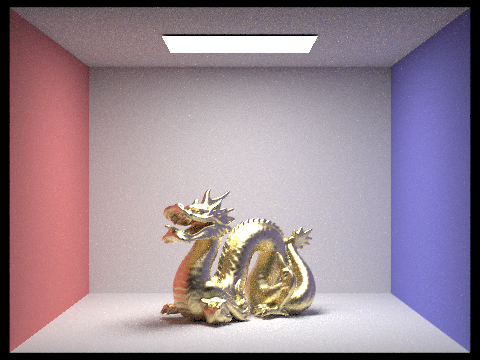
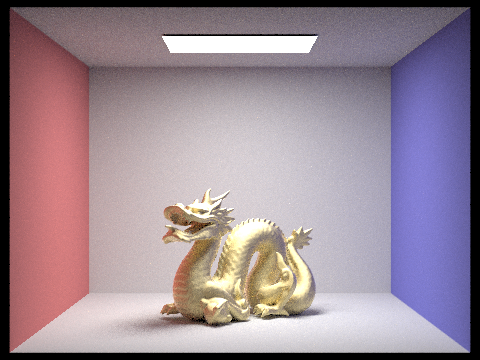
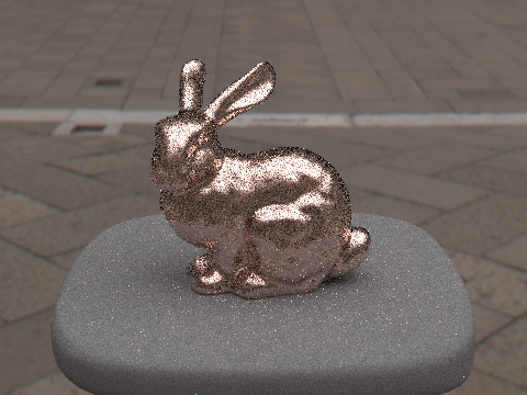
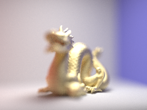
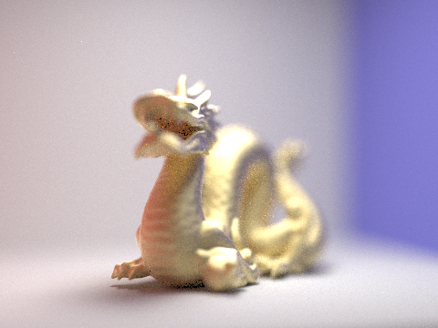
Part 2: Microfacet Material
Below is a series of renderings of dae/sky/CBdragon_microfacet_au.dae with pixel sampling rate at 128 and 1 sample per light.
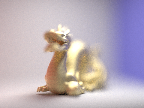
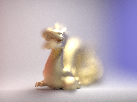
Below is a comparison of dae/sky/CBdragon_microfacet_au.dae between cosine hemisphere sampling and importance sampling, with pixel sampling rate at 64 and 1 sample per light.
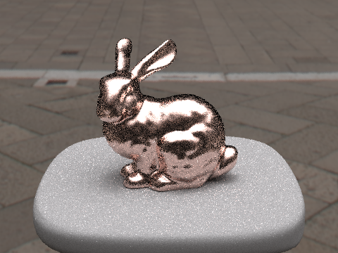
After replacing the $\eta$ and $k$ with those from another conductor material, we can get a different look on the surface.
dae/sky/CBdragon_microfacet_au.dae mesh in titanium.Part 3: Environment Light
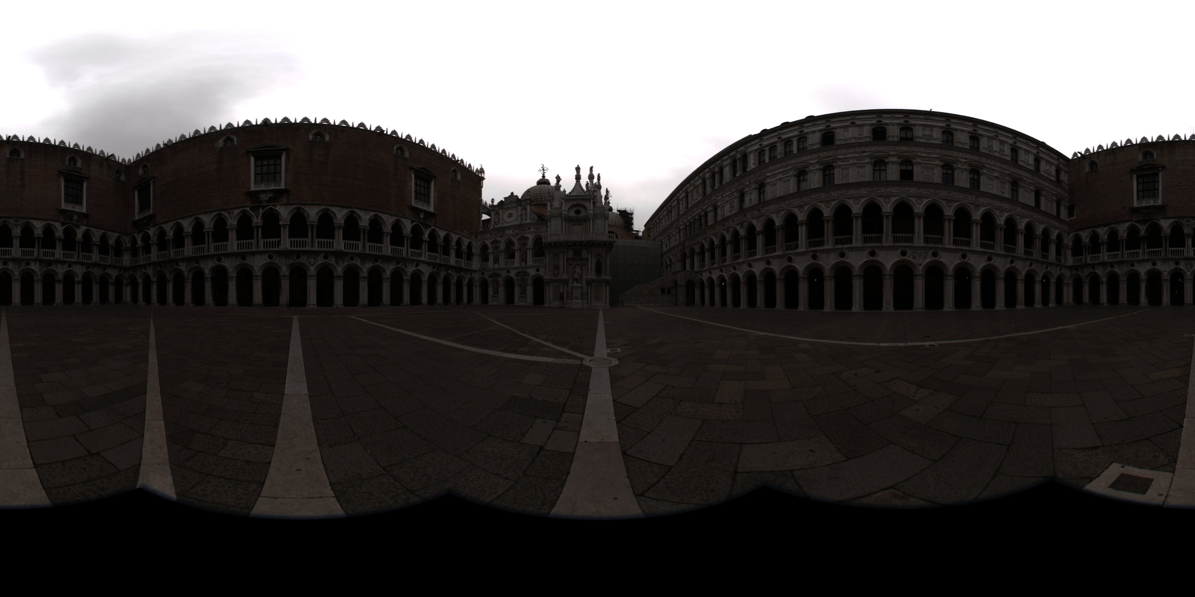
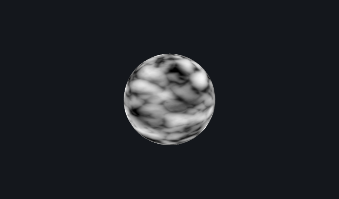
exr/doge.exr.Below is the probability debug file generated based on the environment map for importance sampling later in this part.

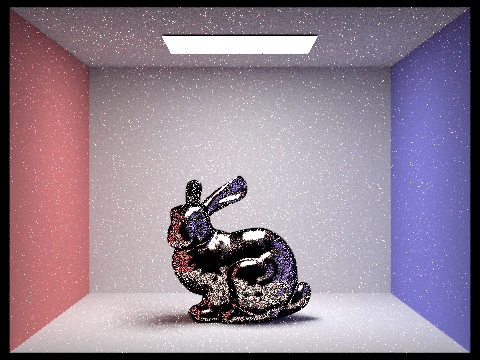
Below is a comparison of dae/sky/bunny_unlit.dae rendered with uniform and importance sampling, pixel sampling rate at 4 and 64 samples per light.
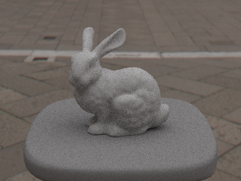
Importance sampling removes some noise from the overall composition. Additionally, it allows the approximation to converge fairly quickly. Around the back of the bunny, we can see a more uniform and brighter look over the area highlight.
Below is a comparison of dae/sky/bunny_microfacet_cu_unlit.dae rendered with uniform and importance sampling, pixel sampling rate at 4 and 64 samples per light.
Importance sampling here allows the highlight area to converge quicker. Since the environment map is very bright over the top area, more samples are drawn with higher probability from there. We can see a significant decrease of noise on the image around the bunny's forehead and back.
Part 4: Depth of Field
Below is a series of renderings of dae/sky/CBdragon_microfacet_au.dae with the virtual camera's focal length at various stops.


Below is a series of renderings of dae/sky/CBdragon_microfacet_au.dae with the virtual camera's aperture at various sizes.
Part 5: Shading
The production-ready release for this part's implementation is available at https://cs184sp18.github.io/proj3_2-pathtracer-sethlu/gl/.
Here I utilized WebGL programs to run interactive graphics apps in the browser. Similar to the OpenGL ES 2.0 specification, each material may be described by a program, typically composed by a vertex and a fragment shader that operates on a per-vertex and per-fragment basis. In a reduced two-stage pipeline, each vertex carying a set of attributes (position, normal, color, texture coordinates, etc.) enters the vertex shader and becomes transformed into normalized device coordinates. After assembling and rasterizing the primitives, each fragment (pixel with interpolated vertex attributes) enters the fragment shader and is either given a color on the framebuffer, otherwise discarded. When coloring each pixel in the framebuffer, lighting functions and textures come into play. Since we know the attributes of the interpolated pixel, we can evaluate lighting functions and sample texture values with the texture coordinates. Additionally, an optional depth test is conducted to check the visibility of the pixel on screen so that a primitive far behind some already painted primitive doesn't overlay the foreground.
Blinn-Phong Shading Model
Below is a breakdown of the different components, with the exponent $p = 100$.

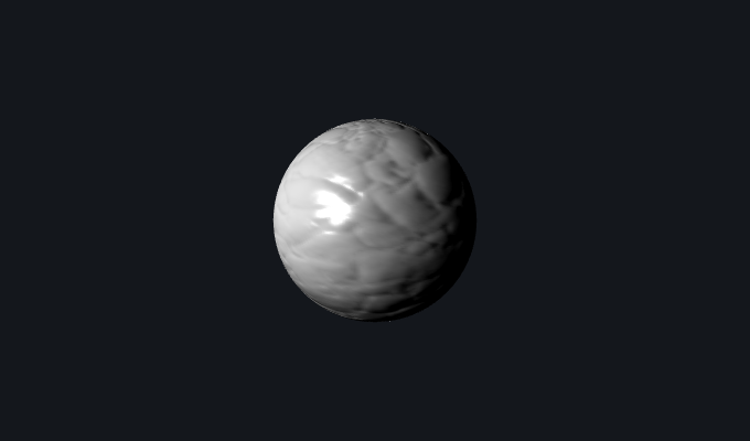
Texture Mapping
Bump & Displacement Mapping
We can implement bump mapping or displacement mapping to achieve more detailed surfaces without sacrificing the vertex count of a scene in the vertex shader. With bump mapping, we can introduce details of the surface without modifying the object geometries—even though the material looks bumpy from the lighting, the surface actually remains the same. Assuming all the surface normals projecting directly outwards from the surface initially, provided with a height map, we can approximate the rate of change on the height of the surface and estimate the surface normals to reflect the heights.
Say locally at a point $p$, the normal vectors points outwards towards $(0, 0, 1)^T$ (in a reference frame local to the point on the surface). We can estimate the surface normal after bump-mapped as $(-dh_{du}, -dh_{dv}, 1)^T$, where $dh_{du} = h(u + 1,v) - h(u, v)$ and $dh_{dv} = h(u, v + 1) - h(u, v)$, when the texture coordinates are aligned with the surface directions. To adjust the contrast of the surface we can optionally multiply $dh_{du}$ and $dh_{dv}$ by some coefficient.


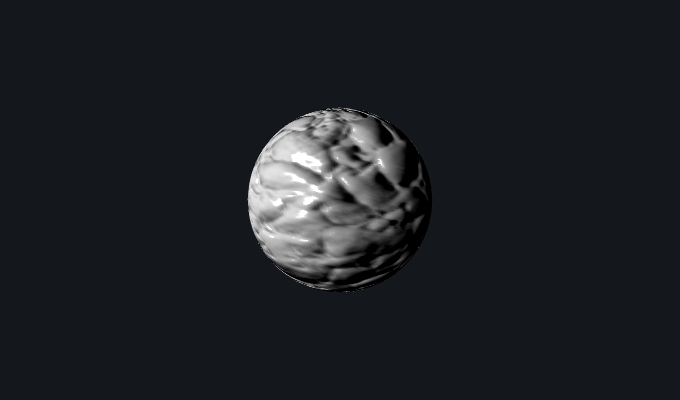
Displacement mapping differs from bump mapping in the way that it actually modifies the geometry of the mesh. We can estimate the surface normal in the same way as in bump mapping, and offset the vertices by the the value from the height map (optionally multiplied by some coefficient to scale the magnitude).


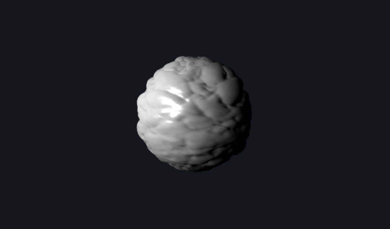
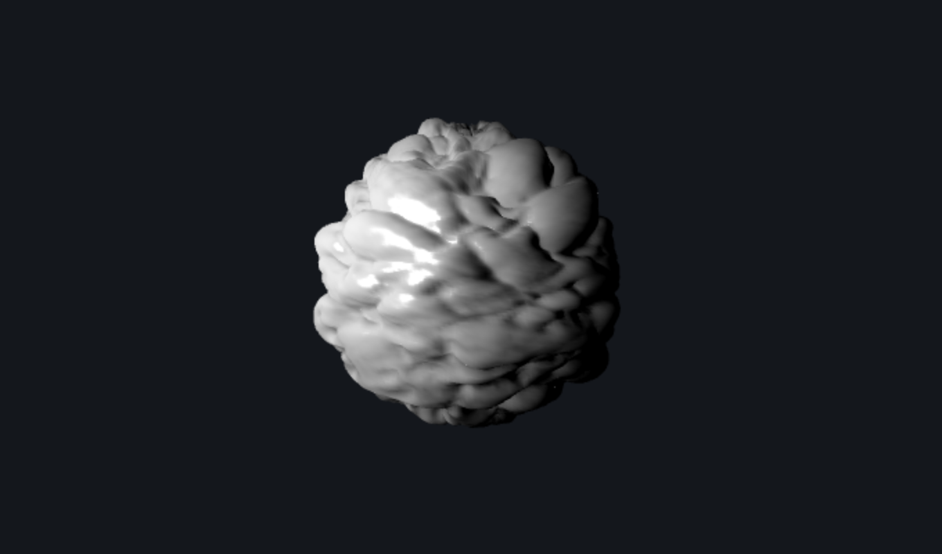
The rubble texture used in this sub-section is retrieved from https://3dtextures.me/2018/01/05/rubble-001/.
Mirror Ball & Environment Map (extra credit)
In this part I implemented a cube environment map and a mirror ball. Here, each fragment over the mirror ball is applied the cube map texture color in the direction of the reflected camera ray. I also surrounded the scene with a cube mesh to create a full coverage over the background, where each fragment is applied the cube map texture in the direction of the camera ray.
The environment map used in this sub-section is retrieved from http://www.humus.name/index.php?page=Textures.