Part 1: Ray Generation and Scene Intersection
Ray Generation
Path tracing begins with a camera. Say, for the camera, we have the bottom left corner as $(0, 0)^T$ and the top right as $(1, 1)^T$. To cast a try from the camera's pinhole through $(x, y)^T$, we can find the normalized 2D camera coordinates for that point by shifting it down left by $(0.5, 0.5)^T$ and scale up the vector by two, resulting in $(2x - 1, 2y - 1)^T$.
Given the field of view of the camera in both $x$ and $y$ directions, $fov_x$ and $fox_y$, we can cast a ray in the camera space from the origin $(0, 0, 0)^T$, in the direction of $((2x-1)\tan(fov_x/2), (2y-1)\tan(fov_y/2), -1)^T$ (that the camera is pointing to negative-$z$), which needs normalizing.
Since path tracing is done in the world space, we need to further transform this ray from the camera space to the world coordinates. Its origin in world coordinates becomes the position of the camera, and its direction can be transformed by the camera's basis matrix for orientation $\begin{bmatrix}\vec{\text{right}} & \vec{\text{up}} & \text{unit}(\vec{\text{pos}_\text{camera}} - \vec{\text{pos}_\text{target}})\end{bmatrix}$, where $\vec{\text{right}}$ can be evaluated from a cross product of $\text{unit}(\vec{\text{pos}_\text{camera}} - \vec{\text{pos}_\text{target}})$ and $\vec{\text{up}}$.
With the method described above we are then able to generate any ray from the camera through $(x, y)^T$. And for every pixel $(x_\text{pixel}, y_\text{pixel})^T$, where at the bottom left pixel it is $(0, 0)^T$ and at the top right it is $(\text{width}_\text{image} - 1, \text{height}_\text{image} - 1)^T$, we can randomly sample a couple of points within the pixel square defined by $(x_\text{pixel}, y_\text{pixel})^T$ and $(x_\text{pixel} + 1, y_\text{pixel} + 1)^T$, at $(x_\text{pixel} + \text{rand}(0, 1), y_\text{pixel} + \text{rand}(0, 1))^T$.
Primitive Intersection
There are two types of primitives covered in this project—triangle and sphere. To test the intersection between a ray and a triangle, we can use the Möller-Trumbore algorithm to solve for the distance between the ray origin and the hit point, and the barycentric coordinates on the triangle. Below is a quick derivation to the algorithm.
Say that the ray is defined as $\vec{r} = \vec{o} + t \vec{d}$, and the triangle is bounded by $\{\vec{a}, \vec{b}, \vec{c}\}$. Since the intersection is on the triangle's plane, we can equate $\vec{r} = \vec{o} + t \vec{d} = (1 - \beta - \gamma)\vec{a} + \beta \vec{b} + \gamma \vec{c}$, where the unknowns are $\{t, \beta, \gamma\}$. After rearranging the equation we can get $t \vec{d} + \beta (\vec{a} - \vec{b}) + \gamma (\vec{a} - \vec{c}) = \vec{a} - \vec{o}$, which can be rewritten as $\begin{bmatrix}\vec{d} & (\vec{a} - \vec{b}) & (\vec{a} - \vec{c})\end{bmatrix}(t, \beta, \gamma)^T = \vec{a} - \vec{o}$. To solve for the unknowns, we can apply an inverse matrix to the left: $(t, \beta, \gamma)^T = \begin{bmatrix}\vec{d} & (\vec{a} - \vec{b}) & (\vec{a} - \vec{c})\end{bmatrix}^{-1}(\vec{a} - \vec{o})$. After some additional simplification, we will end up with the Möller-Trumbore algorithm.
A final step after finding the intersection is to validate its position, whether it's inside the triangle ($0 \leq \beta \leq 1$, $0 \leq \gamma \leq 1$, $0 \leq \beta + \gamma \leq 1$) and it's somewhere in front of the camera ($t > 0$). The ray should intersect the triangle if it passes the test.
Besides intersecting triangles, rays may intersect with spheres as well. The condition for a ray to intersect the surface of a sphere is that $|\vec{r} - \vec{o_\text{sphere}}| = |\vec{o} + t \vec{d} - \vec{o_\text{sphere}}| = r_\text{sphere}$.
The $\Delta$ term in the equation tells how many intersections there are between the ray and the sphere. If $\Delta < 0$, there should be no intersection; if $\Delta = 0$, the ray should be tangent to the sphere; and if $\Delta > 0$, the ray intersects the sphere twice.
Results
Below are the renderings of a few smaller models, shaded by their surface normal vectors.

dae/sky/CBcoil.dae in normal shading.
dae/sky/CBgems.dae in normal shading.
dae/sky/CBspheres_lambertian.dae in normal shading.
dae/keenan/banana.dae in normal shading.Part 2: Bounding Volume Hierarchy
To construct a bounding volume hierarchy (BVH), we begin with a set of primitives. At each level, we select a criteria to partition the set of primitives into two subsets. A heuristic I implemented is to divide the set of primitives at the midpoint of the max spanning axis of those primitives' centroids. For example, given the centroids of three primitives $\{(0, 0, 1)^T, (0, 1, -1)^T, (3, 0, 1)^T\}$, the partition is chosen at the axis-aligned plane where $x = 1.5$. After dividing the set of primitives, we can recursively generate the sub-BVH's for those two subsets of primitives until reaching a desired max primitive count per unit BVH node. It is worth noting that we only store the primitives inside the leaf nodes of the BVH.
An edge case can arise when the primitives share a same centroid. To tackle this issue, I chose to put that primitive into the set that has a smaller size so far.
After constructing a BVH structural representation of the primitives, we can test the intersection of the ray. At each BVH node, we only need to test its bounded primitives if the ray passes through its bounding box. If the ray does intersect the bounding box, for a leaf node we can test all the contained primitives and find the nearest intersection (described in part 1), and for a non-left node, we can recursively test the left and right branches to see of there is a nearest intersection. A gotcha here is that finding a intersection from the left sub-BVH node doesn't mean there isn't a closer intersection from the right sub-BVH.
To test whether a ray passes through a $n$-dimensional bounding box, we can decompose the ray in $n$ dimensions and check if there is an overlapping area across all dimensions. Say for a ray $\vec{r} = \vec{o} + t \vec{d}$, and a bounding box defined by $(x_0, y_0, z_0)^T$ and $(x_1, y_1, z_1)^T$. The ray enters and exits the box in the $x$ direction at $t_{x,0}$ and $t_{x,1}$, in the $y$ direction at $t_{y,0}$ and $t_{y,1}$ and in the $z$ direction at $t_{z,0}$ and $t_{z,1}$. The ray is only inside the bounding box between $t_0 = \text{max}(t_{x,0}, t_{y,0}, t_{z,0})$ and $t_1 = \text{min}(t_{x,1}, t_{y,1}, t_{z,1})$, where a constraint is $t_0 <= t_1$ because it cannot exit a bounding box before it enters.
Results
Below are the renderings of a few relatively more complex models, shaded by their surface normal vectors.

dae/sky/CBlucy.dae in normal shading.
dae/sky/CBdragon.dae in normal shading.
dae/keenan/building.dae in normal shading.
dae/meshedit/maxplanck.dae in normal shading.Performance Comparison
BVH acceleration presents quite a stunning difference in the speed of path tracing. The chart below shows the taken to render the scene with surface normal shading. Note that the measures are marked along a logarithmic scale.
dae/sky/CBlucy.dae, dae/sky/CBdragon.dae, dae/keenan/building.dae and dae/meshedit/maxplanck.dae, tested on Dell Optiplex 9020, Intel quad-core i7-4770 cpu (HT 3.4GHz turbo, 8MB, w/ HD graphics 4600), run with 8 threads.With BVH, we can observe a drastic increase in path tracing performance. Without BVH, it may take up to $1928.9863$ seconds to render dae/sky/CBlucy.dae; with BVH, the time is then reduced to $0.7965$ seconds (about 2400x faster).
Part 3: Direct Illumination
BSDF Shading Model
Begin by first talking about a big picture of direct lighting. When a ray hits a surface, at its intersection all incoming lights will be reflected to the outgoing direction at varying amount. Set the point of intersection as the origin of the reference frame, the surface normal vector as the up direction. We can describe the intensity of the radiance of the outgoing ray (in direction $\omega_o$) as an integration of all incoming irradiance (in direction $\omega_i$) multiplied by how much it contributes to the outgoing radiance.
Recall the definition for irradiance and radiance from a small surface patch:
Note that $dA_\perp = dA \cos(\theta)$, the cosine term being the foreshortening factor, same as in Lambert's cosine law. Now to find the incoming irradiance due to light from $\omega_i$:
We can then write an integration over the surface of the hemisphere to sum all the irradiance contributed from $\omega_i$ towards $\omega_o$: $L_o(\omega_o) = \int_{\Omega} f(\omega_o, \omega_i) \cos(\theta_i) L_i(\omega_i) d\omega_i$. The bidirectional scattering distribution function (BSDF) $f(\omega_o, \omega_i)$ is defined as how much radiance (in the direction of $\omega_o$) is resulted from the irradiance due to light coming from $\omega_i$.
As an example of BSDF, a matte material may be described with a diffuse shading model that reflects incoming light evenly in all directions. In this case the BSDF may also be referred to as bidirectional reflectance distribution model (BRDF) since we only care about the surface reflection without light transmission. Following the uniform reflectivity at all viewing angles, the function $f(\omega_o, \omega_i)$ should stay constant despite that $\omega_o$ and $\omega_i$ may vary, and give the albedo of the material surface $\rho_\text{material}$. For instance, if the irradiance due to $\omega_i$ is $(0.9, 0.5, 0.8)^T$ and that the albedo is $\rho = (0.5, 0, 0)^T$, the resulting radiance in the direction of $\omega_o$ will be $(0.9, 0.5, 0.8)^T * (0.5, 0. 0)^T = (0.45, 0, 0)^T$.
Say we define $f(\omega_o, \omega_i) = \rho$ following the diffuse shading model. If we write out the energy conservation property $\int_\Omega f(\omega_o, \omega_i) \cos(\theta_i) d\omega_i \leq 1$, after integrating we will find $\int_{\Omega} f(\omega_o, \omega_i) \cos(\theta_i) d\omega_i = \int_{\Omega} \rho \cos(\theta_i) d\omega_i = \rho \int_{\Omega} \cos(\theta_i) d\omega_i = \rho \pi \leq 1$. After rearranging we get $\rho \leq \frac{1}{\pi}$. We can choose to normalize $\rho = \frac{\rho_\text{material}}{\pi}$ so that the energy is conserved.
Hemisphere Sampling
Since it is difficult to carry out a precise integration over the hemisphere, we can use Monte Carlo integration to estimate its result. Given the Monte Carlo estimator $F_N = \frac{1}{N} \sum_{i=1}^N \frac{f(x_i)}{p(x_i)}$, we can rewrite the above integration with $\frac{1}{N} \sum_{i=1}^N \frac{f(\omega_o, \omega_i) \cos(\theta_i) L_i(\omega_i)}{p(\omega_i)}$.
For hemisphere sampling, we have a uniform probability distribution $p(\omega_i) = \frac{1}{2 \pi}$ for each incoming direction $\omega_i$. The estimation may then be simplified as $\frac{2 \pi}{N} \sum_{i=1}^N f(\omega_o, \omega_i) \cos(\theta_i) L_i(\omega_i)$. Programmably we can uniformly sample a vector direction over the hemisphere and accumulate the product of its radiance, cosine angle to the surface normal and BSDF. We finally multiply the sum by $2 \pi$ over the number of samples taken.
Importance Sampling
Similar to the hemisphere sampling approach, we instead take samples that prioritize the light sources—a lot of times our randomly chosen rays won't end up hitting the emitting surfaces, resulting in overly dimmed pixels. To address this issue, we sample uniformly over the area lights and weighs each portion differently. For each area light, we can accumulate its contribution to the outgoing radiance at the point of intersection with $\int_{A'} L_i(p, \omega_i) \frac{\cos{\theta} \cos{\theta'}}{|p' - p|^2} dA' = \int_{A'} L_o(p', \omega_i') \frac{\cos{\theta} \cos{\theta'}}{|p' - p|^2} dA'$ when it is not blocked by any primitives in the way.
We can write the Monte Carlo estimator as $\frac{A'}{N} \sum_{i=1}^N L_o(p', \omega_i') \frac{\cos{\theta} \cos{\theta'}}{|p' - p|^2}$ (the probability to arrive on a point on the surface being $p(p') = \frac{1}{A'}$). Again, we need to apply the estimator on each area light to get the final result.
Results
Below are the rendering results from using hemisphere sampling and importance sampling respectively on two scenes.

dae/sky/CBspheres_lambertian.dae rendered with hemisphere shading.
dae/sky/CBspheres_lambertian.dae rendered with importance shading.
dae/sky/CBbunny.dae rendered with hemisphere shading.
dae/sky/CBbunny.dae rendered with importance shading.The number of samples taken per light can greatly affect the quality of final result. Below are the direct lighting results of dae/sky/CBbunny.dae at one camera ray per pixel while at varying sampling rate per area light.


From taking 1 ray and 4 rays per area light, the noise level of the entire scene gets reduced. There is a more defined shaded area under the rabbit; we can see some slight transitions (the gray area) between the floor and the shaded region. From sampling 16 rays to 64 rays per area light, we see a clearer shape of the shadow under the rabbit. Especially around the area of the rabbit's head in the shadow, we see a smoother blending between the light and shadow.
Part 4: Global Illumination
At each surface intersection, not only do we receive direct lighting from emissive objects, but we get indirect lighting from nearby objects as well. When a ray hits a surface, we can randomly cast a ray from the surface intersection and recursively find the incoming radiance from that direction, which would similarly contribute towards the outgoing radiance directed at $\omega_o$.
However, if we keep going down the recursion there would be no base case to stop this process; in my implementation I had a parameter to specify the max recursion depth for a ray. Additionally, I used Russian Roulette to randomly terminate the recursion; the recursion is only applied when the $rand(0, 1) < c$, where $c$ is a probability for termination. To meet the original expectation of the incoming radiance, we would divide the estimated radiance returned from the recursive call by $c$.
Results
Below are some renderings done with global illumination.

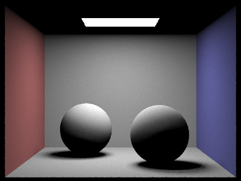
dae/sky/CBspheres_lambertian.dae rendered at pixel sampling rate of 4, 64 samples per area light at a max recursion depth of 6.
dae/sky/CBbunny.dae rendered at pixel sampling rate of 4, 64 samples per area light at a max recursion depth of 6.Direct vs Indirect Lighting
Indirect lighting brings some brightness to areas that are not directly reachable by the light source. Below is a side-by-side comparison of dae/sky/dragon.dae between only direct (max one bounce) and only indirect lighting.

In the direct lighting result, we only see a blank and white representation of the spheres. However, in the indirect lighting result shown on the right, there are more colors introduced to not only the lit areas but also the shadows. There is light indirectly from the light sources that contributes to the outgoing radiance.
Increasing Max Ray Depth
Below is a series of renderings of dae/sky/CBbunny.dae showing the progression of an increasing max recursion depth for the camera ray.


Without any light bounce, only radiance directly from the self-emissive objects are perceived. At max ray depth 1, we get the direct shading as described in the previous section. The scene gets a little more interesting as we walk to higher max ray depth. Starting from a max depth of 3, we can begin to see indirectly lit colors of the walls from two sides in the shadows of the object.
Increasing Pixel Sampling Rate
Below is a series of renderings of dae/sky/dragon.dae done at various stops of pixel sampling rates at 4 ray samples per area light.


From having a pixel sampling rate at 1 to 1024, there is a drastic increase in the clarity of the rendered product; there is little graininess in the highest sampling rate version. The surfaces are smoother, and the shadows are more defined.
Part 5: Adaptive Sampling
For an area that's outside the Cornell box, it would be quite a waste to sample those pixels the same amount as the other ones which have more details. In generalization, there are pixels on the image that don't require very detailed sampling.
To adapt to rays sampled per pixel, we can dynamically choose to terminate per-pixel path tracing depending on how confident we are with the result accumulated so far. Here we use z-test measure the pixel's convergence.
To begin with, we can keep a running sum for each sample's illuminance in $s_1$ and for each squared illuminance in $s_2$. After having taken $n$ samples we can find the mean and the variance of the samples with $\mu = \frac{s_1}{n}$ and $\sigma^2 = \frac{1}{n - 1}(s_2 - \frac{s_1^2}{n})$.
Then we can find the standard error $SE = \frac{\sigma}{\sqrt{n}}$, and get a confidence interval of $\mu \pm z * \frac{\sigma}{\sqrt{n}}$. To be $95\%$ confident with the sampled result, we get an interval $\mu \pm 1.96 \frac{\sigma}{\sqrt{n}}$. Say we tolerate $5\%$ of that condifdence interval regarding the sampled mean: If we satisfy $1.96 \frac{\sigma}{\sqrt{n}} \leq 0.05 \mu$, we are pretty sure about the solution.
Results
Below are the results of dae/sky/CBspheres_lambertian.dae both from adaptive sampling and sampling normally with a 1024 pixel sampling rate, where the blue regions represent where the least samples are taken, the red regions being where the most samples are taken.


Adaptive sampling doesn't introduce many artifacts; one notable one from the results shown above is over on the sphere on the right. There is one point that is darker than the rest of the surface due to an early convergence—the corresponding pixel on the right shows a tiny blue pixel.