CS 184: Computer Graphics and Imaging, Spring 2018
Project 2: Mesh Editor

Zhuo Lu (Seth), cs184-aea

Section I: Bézier Curves and Surfaces

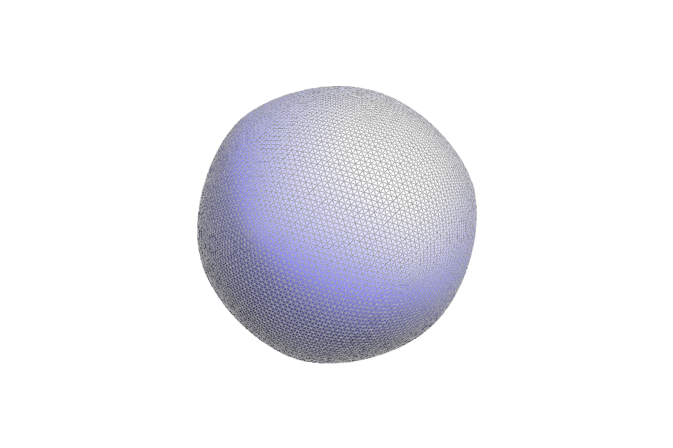
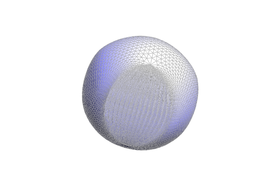
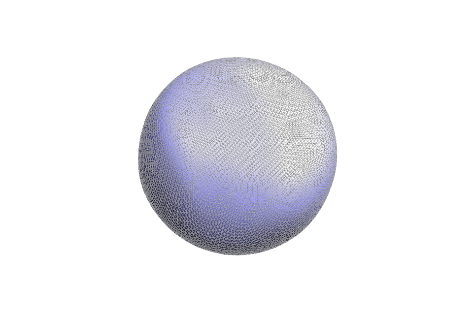
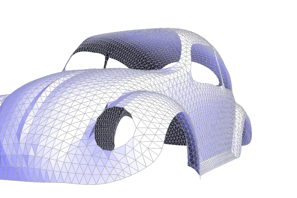
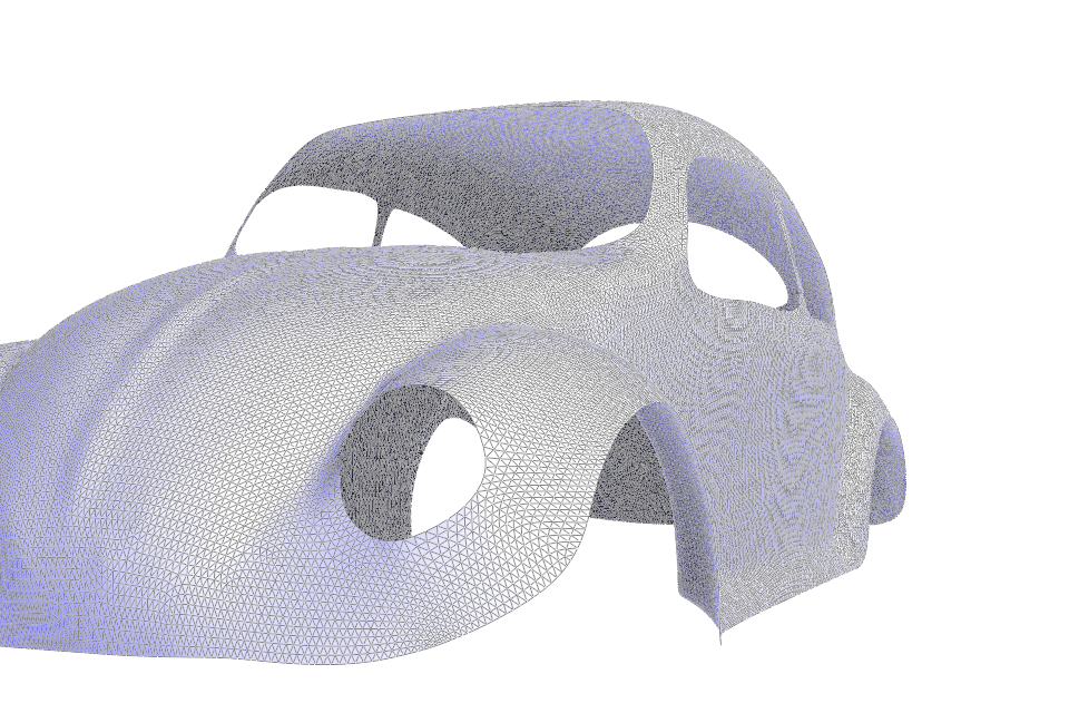
In this project I managed to implement de Casteljau's algorithm for Bézier curve and patch interpolation. Additionally, I implemented a few methods that operate on half-edge meshes (fairly direct topological representation of models): To flip and to split edges; and, based on those two, to Loop subdivide a mesh. Through the course of the project, I learned a half-edge data structure to store geometry information, and gained a better understanding of Loop subdivision. It is also very rewarding to see the implementation in action towards the end, especially it being able to take a scene exported from Blender and to render it in real time!

Part 1: Bézier curves with 1D de Casteljau subdivision

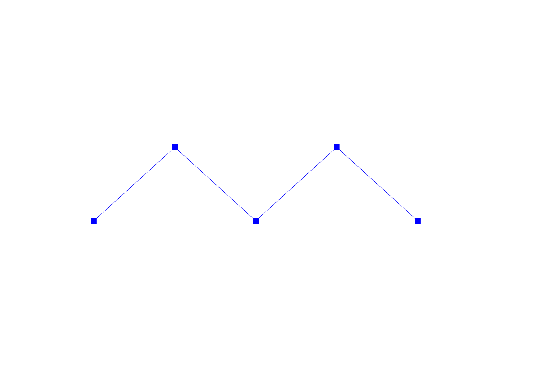
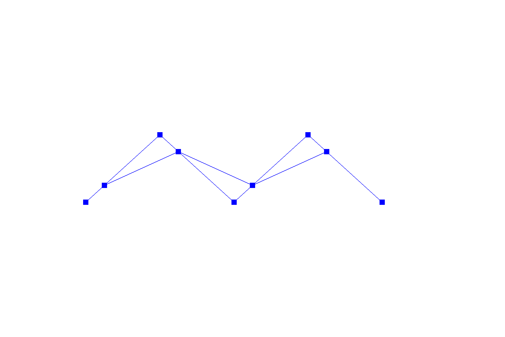
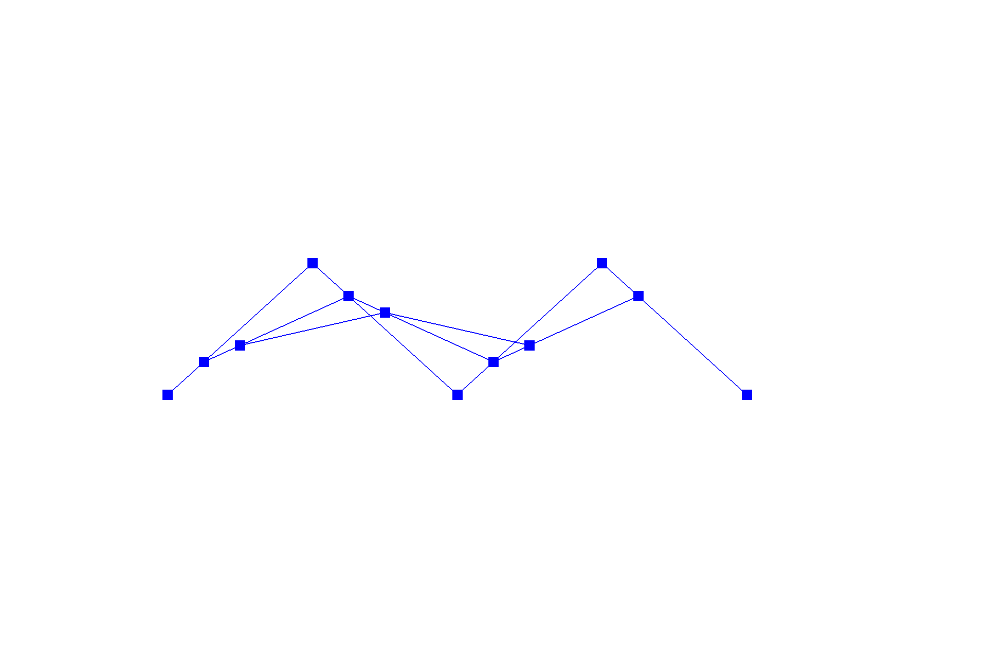
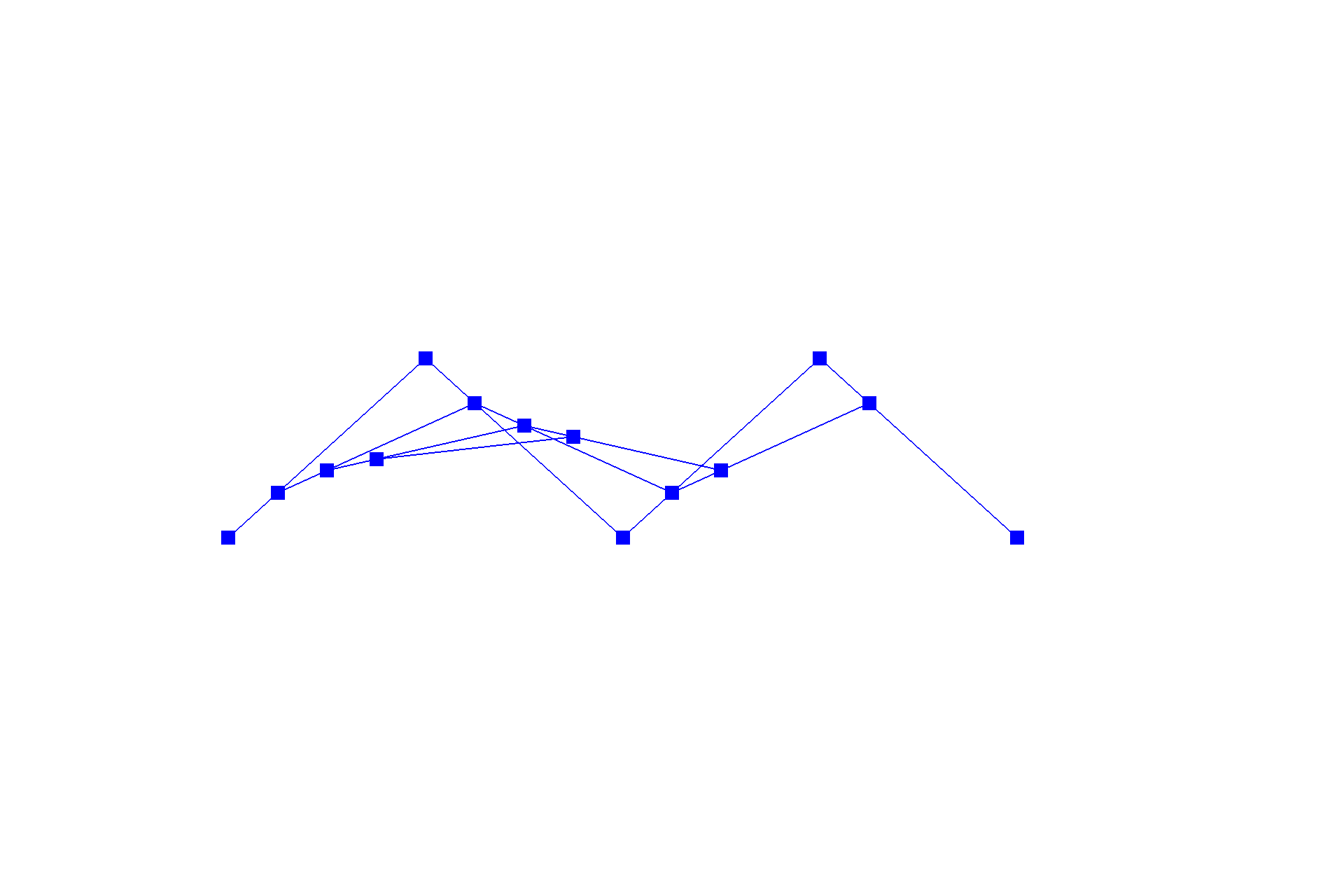
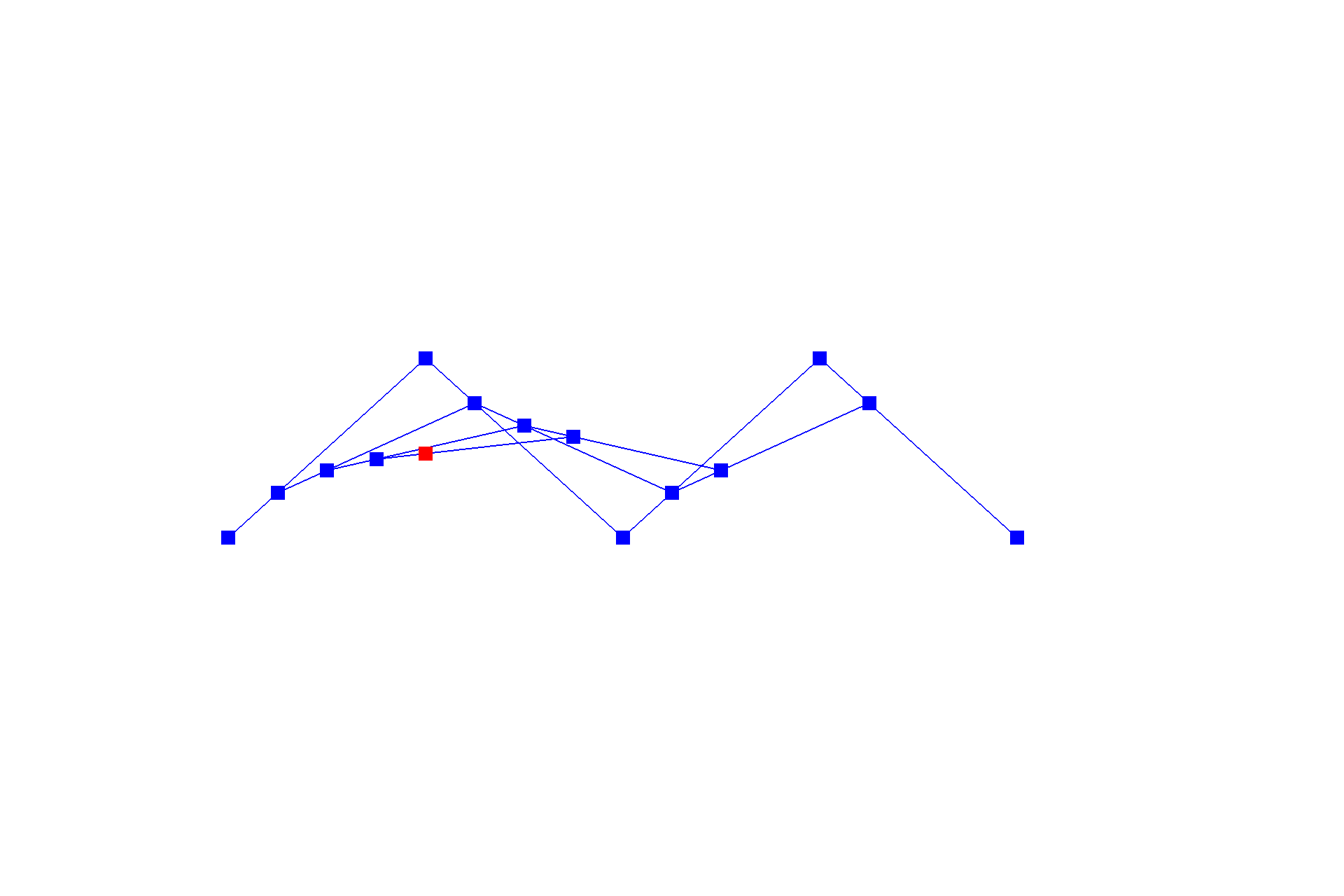
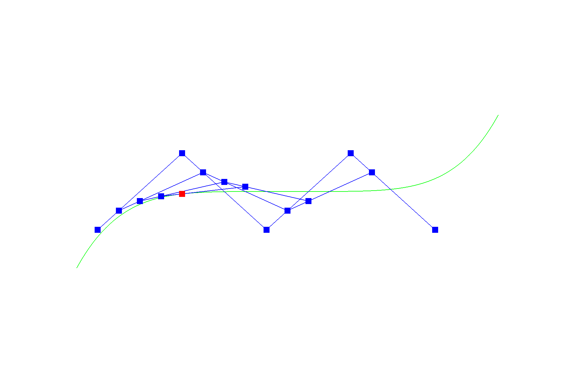
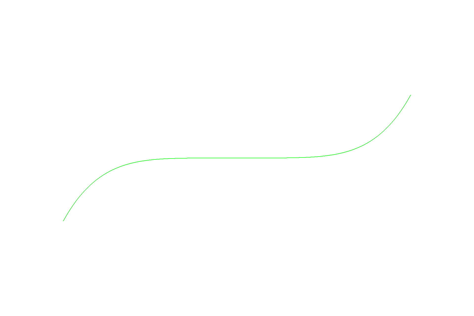
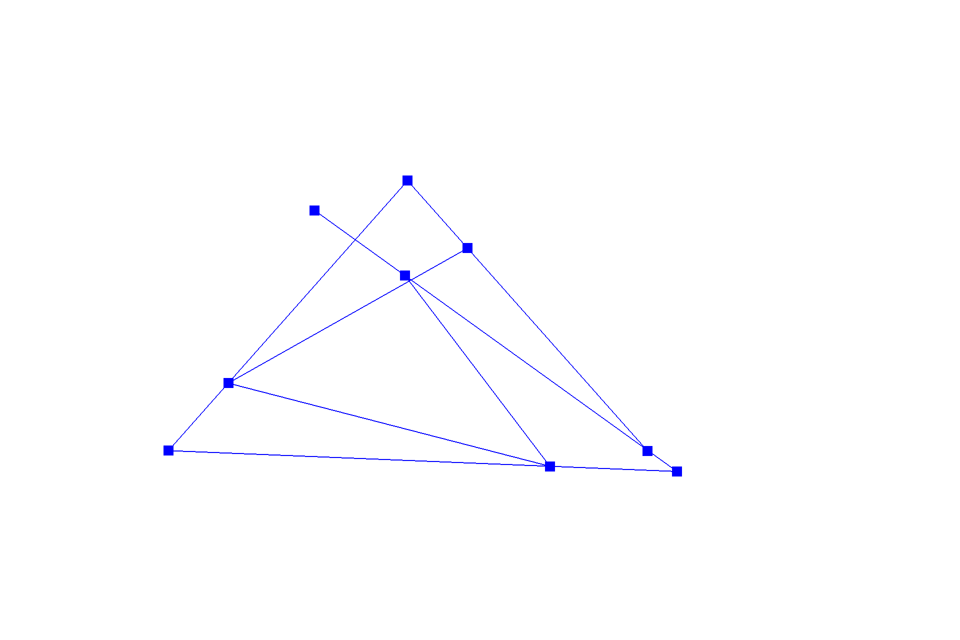
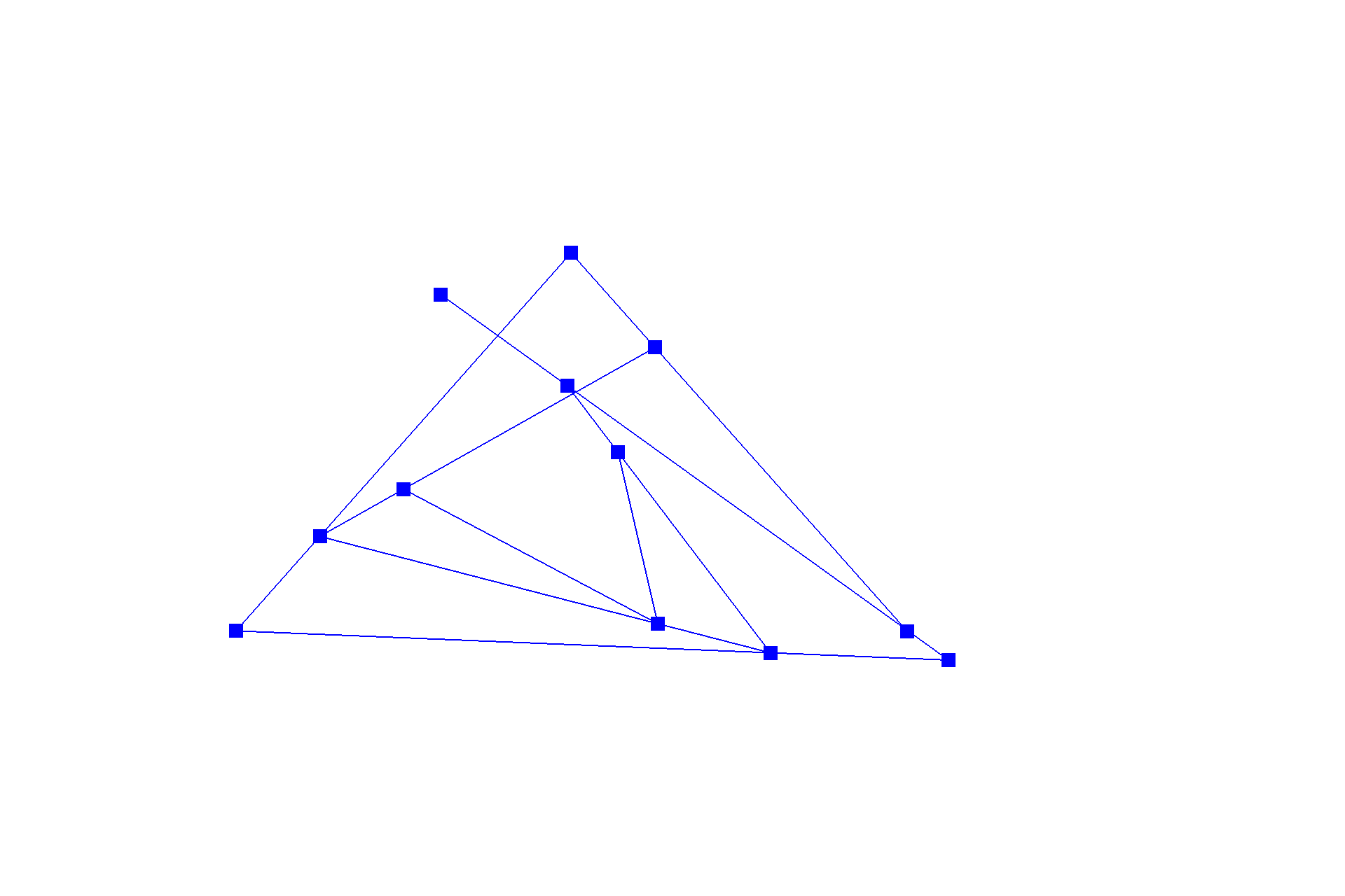
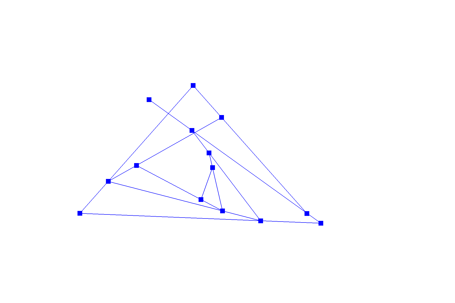
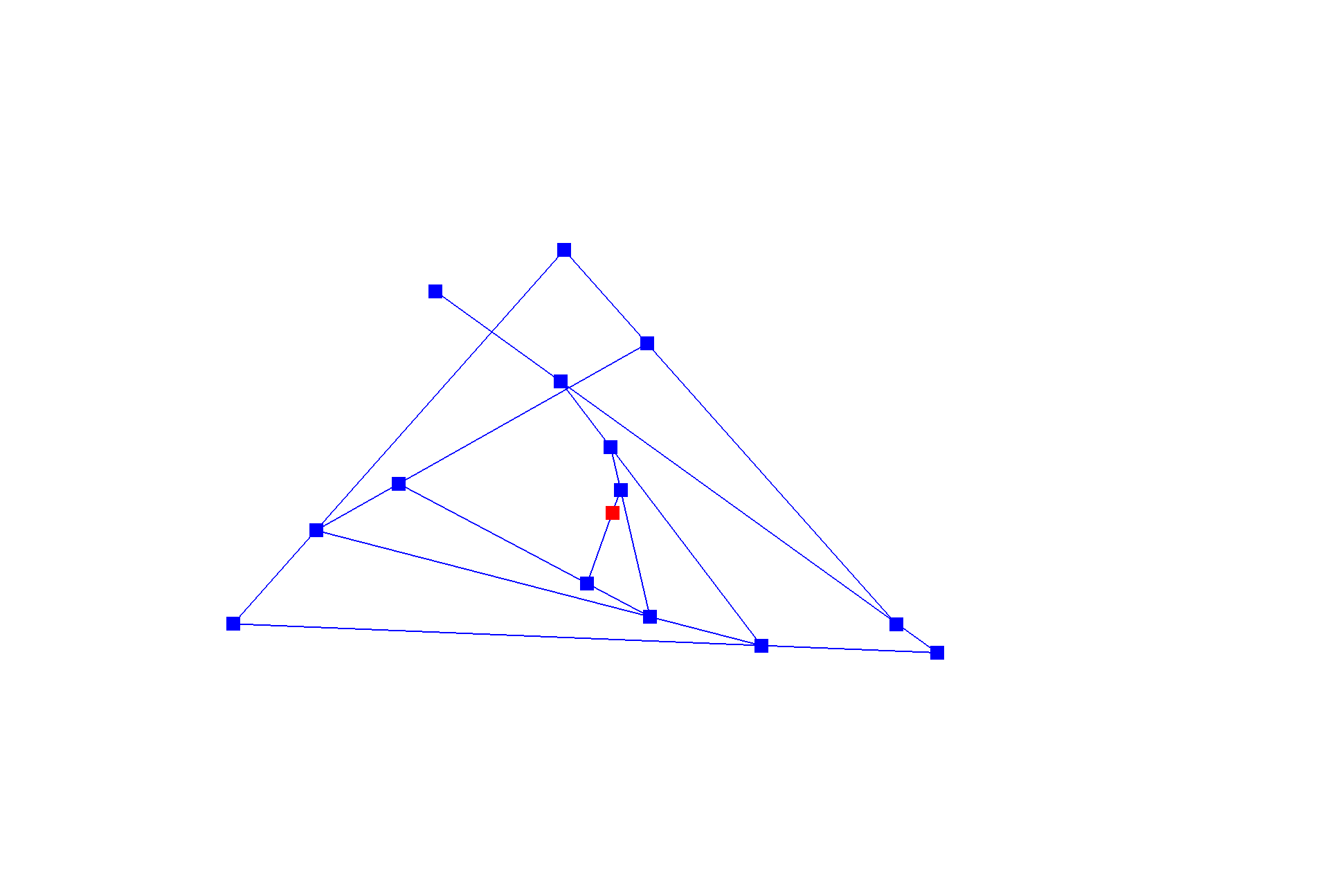
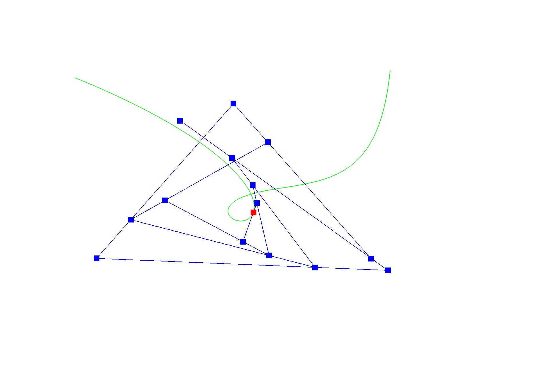
De Casteljau's algorithm is one method to evaluate a point on a Bézier curve with recursion. It starts with an initial series of $n$ control points $\{p_0, p_1, ... , p_{n-1}\}$, and recursively linearly interpolates each segment $\{\{p_0, p_1\}, \{p_1, p_2\}, ... , \{p_{n-2}, p_{n-1}\}\}$ by a factor of $t$ (like convolution in one dimension), reducing the number of control points by one, resulting in $\{(1-t) * p_0 + t * p_1, (1-t) * p_1 + t * p_2\, ... , (1-t) * p_{n-2} + t * p_{n-1}\}$, until there be one point left in the set. Following this scheme, we can naively interpolate a Bézier curve by sampling multiple points on the curve at different $t$'s. Below shows a progression from the original series of six control points to the resulting curve.

Bézier curve with 6 control points. Move the slider to see different stages of this algorithm in action at $t = 0.25$.

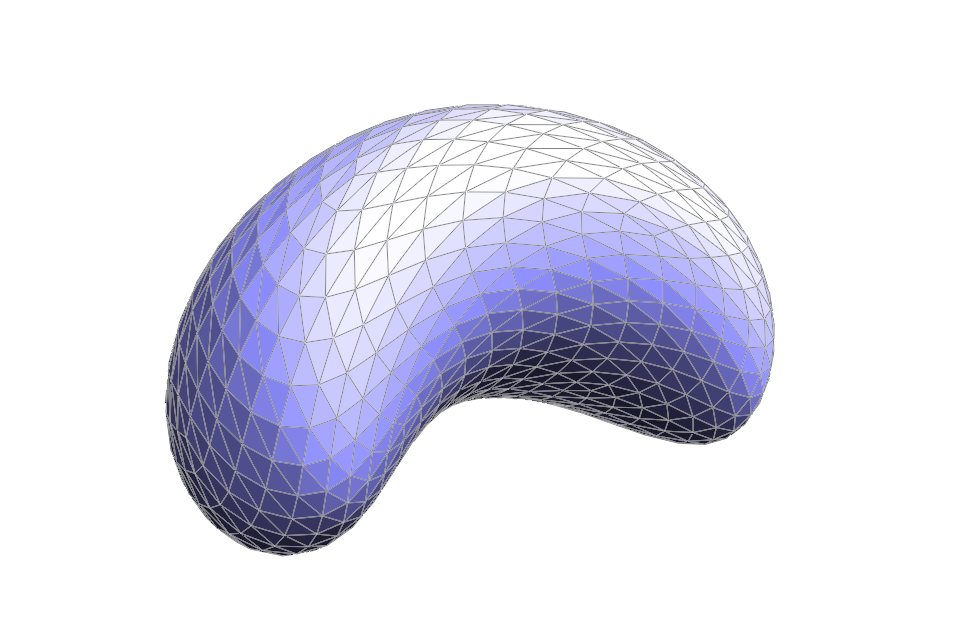
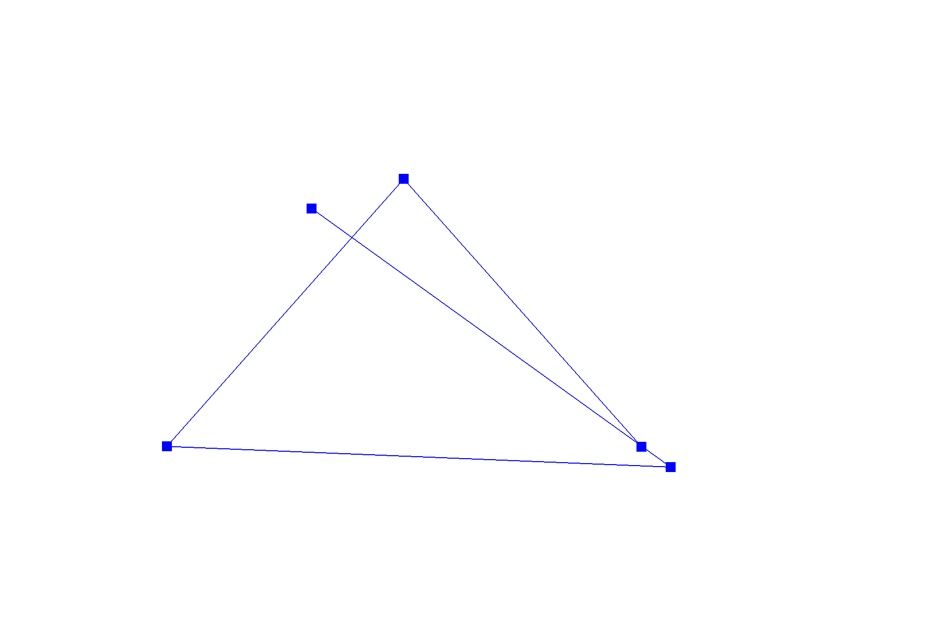
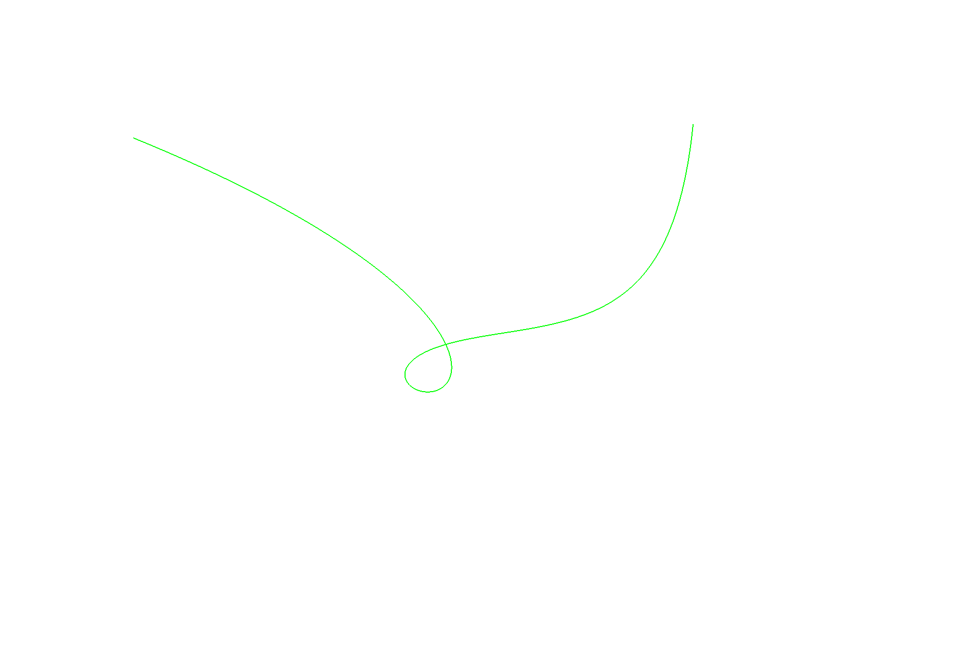
By moving those control points around, we can create a loopy shape with Bézier curve too.

Another Bézier curve with 6 control points at $t = 0.75$. The shape it creates can be fairly elaborate.

Part 2: Bézier surfaces with separable 1D de Casteljau subdivision

Beyond Bézier curves, we can interpolate Bézier patches with de Casteljau's algorithm as well. To give an example of a surface defined by $16$ control points, $\{p_{0,0}, p_{0,1}, p_{0,2}, p_{0,3}, p_{1,0}, p_{1,1}, p_{1,2}, p_{1,3}, p_{2,0}, p_{2,1}, p_{2,2}, p_{2,3}, p_{3,0}, p_{3,1}, p_{3,2}, p_{3,3}\}$. We can first interpolate parallel lines on the surface defined by $\{p_{0,0}, p_{0,1}, p_{0,2}, p_{0,3}\}$, $\{p_{1,0}, p_{1,1}, p_{1,2}, p_{1,3}\}$, $\{p_{2,0}, p_{2,1}, p_{2,2}, p_{2,3}\}$ and $\{p_{3,0}, p_{3,1}, p_{3,2}, p_{3,3}\}$; at factor $u$, we get $4$ intermediate control points $\{p_{0,0}^{0,3}, p_{1,0}^{1,3}, p_{2,0}^{2,3}, p_{3,0}^{3,3}\}$ (like on a cross section of the surface). With those intermediate control points, we can further interpolate the curve at that cross section by varying another factor $v$ to get a point on the Bézier surface $p_{0,0}^{3,3}$. The $v$ here does a similar job to $t$ in part one.

Also, it does not matter in which order the two-part-interpolation is carried out. We can choose to first interpolate with $\{p_{0,0}, p_{1,0}, p_{2,0}, p_{3,0}\}$, $\{p_{0,1}, p_{1,1}, p_{2,1}, p_{3,1}\}$, $\{p_{0,1}, p_{1,2}, p_{2,2}, p_{3,2}\}$ and $\{p_{0,3}, p_{1,3}, p_{2,3}, p_{3,3}\}$ at $v$ to get intermediate control points $\{p_{0,0}^{3,0}, p_{0,1}^{3,1}, p_{0,2}^{3,2}, p_{0,3}^{3,3}\}$. Afterwards, with those intermediate points we can further interpolate a point on the surface $p_{0,0}^{3,3}$ at a factor $u$.

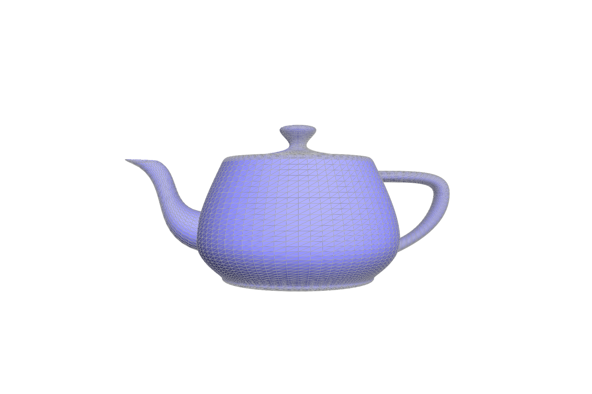
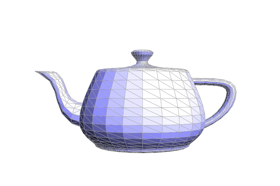
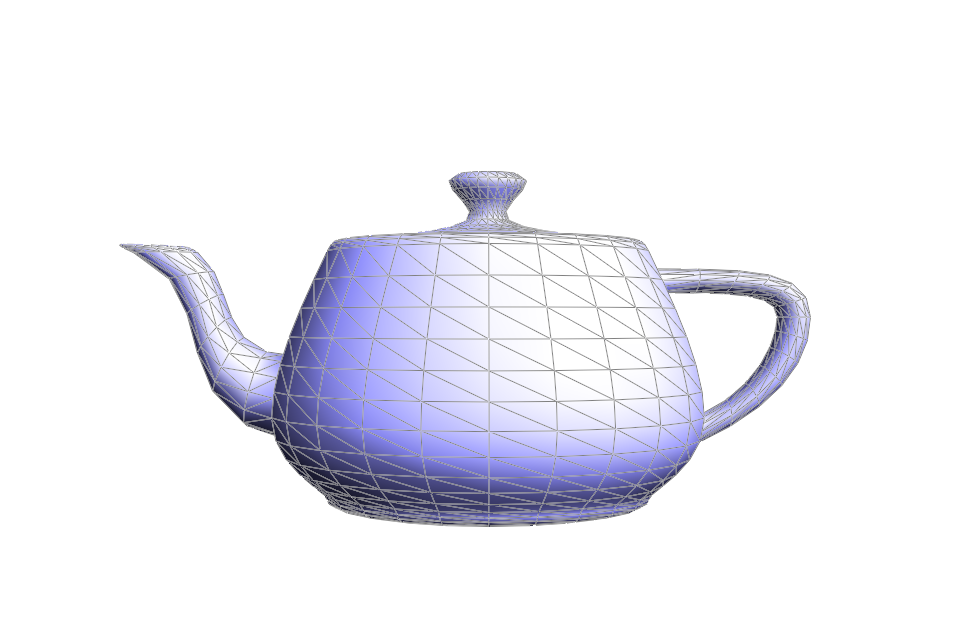
Below is an example with Bézier surfaces interpolated with the above algorithm.

The Utah teapot with wire frames in flat shading.

Section II: Loop Subdivision of General Triangle Meshes

Part 3: Average normals for half-edge meshes

In this part, I implemented a vertex normal approximation based off the vertex's neighboring triangular faces that would allow smooth surface shading. In finer detail, it takes a weighted average of the neighboring face normals with respect to their areas. At a vertex $\vec{v}$, we can discover one of its outgoing half edge $h_0$; following this half edge we can find the vertices $\{\vec{v}_0, \vec{v}_1, \vec{v}_2\}$ that define the triangle, to which the half edge $h_0$ belongs, and can calculate the face normal by taking a cross product of $\vec{v}_0 - \vec{v}_1$ and $\vec{v}_2 - \vec{v}_1$. The area of the triangle is half of the magnitude of the cross product. After iterating through the triangles around the vertex $v$ we can find the sum of face normals and that of face areas too. For completeness of explanation, we can move from one outgoing half edge to a next by finding its twin's next half edge.

To optimize the computation slightly, we can postpone the intermediate vector normalization and weighing for each face until after processing all the faces:

\begin{align*} \vec{n} & = \frac{\sum_{f \in \text{faces}} \hat{f_\text{normal}} * f_\text{area}}{\sum_{\text{face} \in \text{faces}} f_\text{area}} \\ & = \frac{\sum_{f \in \text{faces}} \frac{f_\text{normal}}{2 f_\text{area}} * f_\text{area}}{\sum_{f \in \text{faces}} f_\text{area}} \\ & = \frac{\sum_{f \in \text{faces}} \frac{1}{2} f_\text{normal}}{\sum_{f \in \text{faces}} f_\text{area}} \\ & = \frac{\sum_{f \in \text{faces}} f_\text{normal}}{2 \sum_{f \in \text{faces}} f_\text{area}} \end{align*} \begin{align*} \hat{n} & = unit(\frac{\sum_{f \in \text{faces}} f_\text{normal}}{2 \sum_{f \in \text{faces}} f_\text{area}}) \\ & = unit(\frac{\sum_{f \in \text{faces}} f_\text{normal}}{\sum_{f \in \text{faces}} f_\text{area}}) \end{align*}

The produced result is shown below:

The Utah teapot with wire frames in flat versus smooth shading.

Part 4: Half-edge flip

The edge flip function takes a non-boundary edge and reconnects the edge to the opposing vertices against the edge provided instead. Below is an illustration of the change in relationships between half-edges $\{h_0, ... h_5\}$, vertices and faces $\{f_0, f_1\}$. To give an example of each type of change, for the half-edge $h_0$, its new next half-edge becomes $h_4$ and its vertex becomes the same as that of $h_5$, its twin, edge and face staying the name. The vertex for $h_0$ before flipping needs $h_3$ as its new half-edge. For face $f_0$, its halfedge needs to be one of $\{h_0, h_4, h_3\}$ after edge flipping; before, it may be one of $\{h_0, h_2, h_4\}$.

Helper diagram I used during the implementation of this feature.

For the implementation, I first exhaustively set pointers to all of the half-edges $\{h_0, ... , h_5\}$. Then, I just reassigned each of the properties for the half-edge to its new state, also taking care of updating the vertices that $h_0$ and $h_1$ connects to before flipping and updating the half-edges for the two faces.

A trick I used while implementing the function is to utilize Halfedge::setNeighbors(HalfedgeIter, HalfedgeIter, VertexIter, EdgeIter, FaceIter) to set every possible properties of the half-edges; it is better to cover all the property updates than to prematurely optimize the code. To debug the integrity of the mesh after edge flipping, I would manually counter-check the element properties (pointer values) and see, for example, whether the half-edge the face points to is actually on the face itself. The rendering result is shown below.

Comparison of dae/bean.dae before and after flipping some edges.

I didn't embark onto an eventful debugging journey while initially implementing this feature; however, later when working on part six, I found myself changing two lines of the code in this part that I thought I had made a typo. Afterwards I returned to working on part six. When the result from part six began to look weird, like faces crossing over each other, it took me about an hour to realize that I did not verify the changes made in this function which caused the issue. What I learnt: The vertex of a half-edge is its originating vertex, not the one it points to.

Part 5: Half-edge split

Below is a diagram I used while implementing the half-edge split. I initially set pointers to the new half-edges $\{h_6, ... , h_{11}\}$, to the new vertex inserted around the midpoint of the edge being split, to each of the three new edges and to the existing and the new faces $\{f_0, ... , f_3\}$. Then I went through each of these elements and update its relations to the neighboring ones.

Helper diagram I used during the implementation of this feature. New half-edges, vertices, edges and faces are highlighted in blue.

For instance, the half-edge $h_8$'s vertex will point to the newly inserted vertex at the center, its next half-edge will be $h_2$, its twin half-edge will be $h_1$, its edge will point to a newly inserted edge and its face will point to $f_2$. For the newly inserted vertex, its halfedge could be any of $\{h_8, h_9, h_{10}, h_{11}\}$. Again, an implementation trick I used is to update as comprehensively as possible all attributes before optimizing. Otherwise, it is likely that something ends up not updated. With that, I didn't go on an epic debugging quest for this part.

Below is a pair of screenshots of the result after some edge splits.

Comparison of dae/quadball.dae before and after splitting some edges.

Edge splits are compatible with edge flips. Below is a pair of screenshots of the result after a combination of both edge splits and flips.

Comparison of dae/quadball.dae before and after splitting and/or flipping some edges.

I also implemented edge splits along boundary edges. Below is a pair of screenshots of this feature in action.

Comparison of dae/beetle.dae before and after splitting some boundary edges.

Part 6: Loop subdivision for mesh upsampling

My implementation of Loop subdivision can be broken down into four distinct steps. Each step is demonstrated in the slides below.

  1. Pre-compute positions for the existing vertices and for the new ones;
  2. Split all existing edges;
  3. Flip new edges that touches an old vertex;
  4. Assign all vertices with their new positions.
Mesh at each of the 4 steps of Loop subdivision implemented.

For an existing or new non-boundary vertex, its new position will be a weighted average of the positions of the surrounding vertices. An existing vertex of degree $n$ will a weight of $u = \frac{3}{16}$ if $n = 3$ or $u = \frac{3}{8n}$ otherwise for its neighboring vertex positions, and $1 - n*u$ for its current position. A newly inserted vertex along a shared edge of two triangles will have a weight of $\frac{3}{8}$ for positions of vertices along the edge, and $\frac{1}{8}$ for the furthest vertices' positions.

An implementation trick I used is to step through each of these steps and make sure the result is consistent with what's expected. It is a little easier to debug this part as its implementation details are heavily dependent on the previous two and it's a little easier to see the bigger picture.

On the result it produces, quite noticeably, after Loop subdivision, the sharp corners and edges disappear while the mesh shrinks slightly in size.

Original icosahedron.
Original icosahedron after 4 times Loop subdivision.

To preserve some of the sharp corners and edges, I found it quite effective to pre-subdivide areas that need sharper details. The bottom right result presents a flat surface from the pre-subdivided triangular surface.

Pre-processed icosahedron with edge splitting along an edge.
Pre-processed icosahedron with edge splitting along an edge after 4 times Loop subdivision.
Pre-processed icosahedron.
Pre-processed icosahedron after 4 times Loop subdivision.
Pre-processed icosahedron with more subdivision.
Pre-processed icosahedron with more subdivision after 4 times Loop subdivision.

An issue with Loop subdivision comes in when the topological model of the mesh doesn't well represent the geometry. For the symmetric mesh in dae/cube.dae, due to the asymmetric topology, the repeatedly subdivided mesh can result in a loss of symmetry. Below is the mesh before and after 4 times Loop subdivision.

Original cube.
Original cube after 4 times Loop subdivision.

To alleviate the asymmetry in the result geometry, we can preprocess the topology to be more symmetric while retaining the same geometry. The pair of screenshots below shows the mesh before and after 4 times Loop subdivision. On the left is the preprocessed mesh (by splitting the edge on each face once), with each face having 4 rotationally symmetric triangles. Now, the subdivided mesh is in better symmetry.

Pre-processed cube.
Pre-processed cube after 4 times Loop subdivision.

Special case at mesh boundary (extra credit)

For the completeness of Loop subdivision, the implementation is also expected work with meshes with boundaries (creases), which add a special case for updating vertex positions.

Comparison of dae/beetle.dae before and after 2 times Loop subdivision.

Section III: Art Competition

Part 7: Draw something interesting!

I thought making a pumpkin would be quite fun, so I ended up designing a single pumpkin, topologically equivalent to a UV-sphere. Then I used particle system to generate a bunch of those pumpkins.

The mesh before and after 2 times Loop subdivision.

I customized two additional shaders following modeling the scene. (However, they are not really meant for generic use.) And the results are shown below:

In a Yayoi Kusama style (but you see thru the faces) and in abstract stripes, both shaded with a custom Lambertian reflectance model. Background color added for final composition, both of the renderings have transparent background.