CS 184: Computer Graphics and Imaging, Spring 2018 Project 1: Rasterizer
Zhuo Lu (Seth), cs184-aea
Section I: Rasterization
The 2D coordinate system in this write-up is defined as that the origin sits at the top left corner, $x$-direction pointing to the right, $y$-direction pointing down.
Part 1: Rasterizing single-color triangles
I started off with sampling the bounding box of the triangle, which is only better than sampling every single screen pixel. The process to rasterize each triangle is to first find its bounding box, defined by its minimum/maximum $x$ and $y$ coordinates. For example, a triangle with vertices $\{(160.944, 290.618)^T, (189.263, 682.358)^T, (53.3333, 486.489)^T\}$ can be contained in a rectangle with its top left corner at $(x_\text{min}, y_\text{min})^T = (53.3333, 290.618)^T$ and its bottom right corner at $(x_\text{max}, y_\text{max})^T = (189.263, 682.358)^T$.
Then, for every pixel in this bounding box, we can test whether it lies within the triangle: We can test whether a point is to the left of a line defined by $\vec{r} = \vec{a} + \lambda \vec{d}$, where $\vec{a}$ is any position along the line and $\vec{d}$ is its normalized direction. To take a normal to the 2D line, at a $90$-degree angle counter clockwise, we can left multiply $\begin{bmatrix}0 & -1 \\ 1 & 0\end{bmatrix}$ ($90$-degree CCW rotation) to $\vec{d}$ and get $\vec{n}$, a normalized normal vector to the line. Now, to test whether a point $\vec{p}$ is to the left of the line, we can define function $L(\vec{p}) = \vec{n} \cdot (\vec{p} - \vec{a})$.
To test if a point is contained in the triangle, we only need to check if the point lies on the same side of all edges. For point $\vec{p}$, we test whether its leftness/rightness of an edge between $\vec{u}$ and $\vec{v}$ with function
If it's the case that $\{L(\vec{p}, \vec{v_0}, \vec{v_1}), L(\vec{p}, \vec{v_1}, \vec{v_2}), L(\vec{p}, \vec{v_2}, \vec{v_0})\}$ are on the same sides (all having the same sign), then the point is contained in the triangle. However, the words here are a little fuzzy. To clarify: Assume $\{v_0, v_1, v_2\}$ are defined in CCW order, $L(\cdot)$ for every input greater than $0$ means the point is contained in the triangle because it is to the left of every edge. However, it could also be the case that $\{v_0, v_1, v_2\}$ are defined in CW order, then $L(\cdot)$ for every input less than $0$ means the point is contained in the triangle because it is to the right of every edge. The edge case is when $L(\cdot)$ is zero.
With that, we can experiment with each pixel. Back to the example earlier, to iterate through every pixel in the bounding box, we can loop over $\{(x, y)^T | x \in [floor(x_\text{min}), floor(x_\text{max})], y \in [floor(y_\text{min}), floor(y_\text{max})]\}$, which is the same as $\{(x, y)^T | x \in [floor(x_\text{min}), ceil(x_\text{max})), y \in [floor(y_\text{min}), ceil(y_\text{max}))\}$, that's used in the renderer implementation.
Since for every pixel, its center is offset by $0.5$ in both $x$ and $y$ directions, each sampling will be made at $\{(x + 0.5, y + 0.5)^T | x \in [floor(x_\text{min}), ceil(x_\text{max})), y \in [floor(y_\text{min}), ceil(y_\text{max}))\}$.
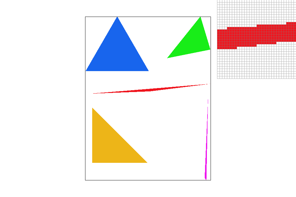
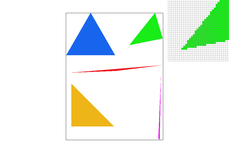
First attempt to rasterize triangles with their bounding boxes.
Slight optimization (extra credit)
In addition to the bounding approach, I attempted to implement a slightly quicker scanning method by splitting triangles to top and bottom halves (two flat triangles) and conduct a more predictive scanning over the shape.
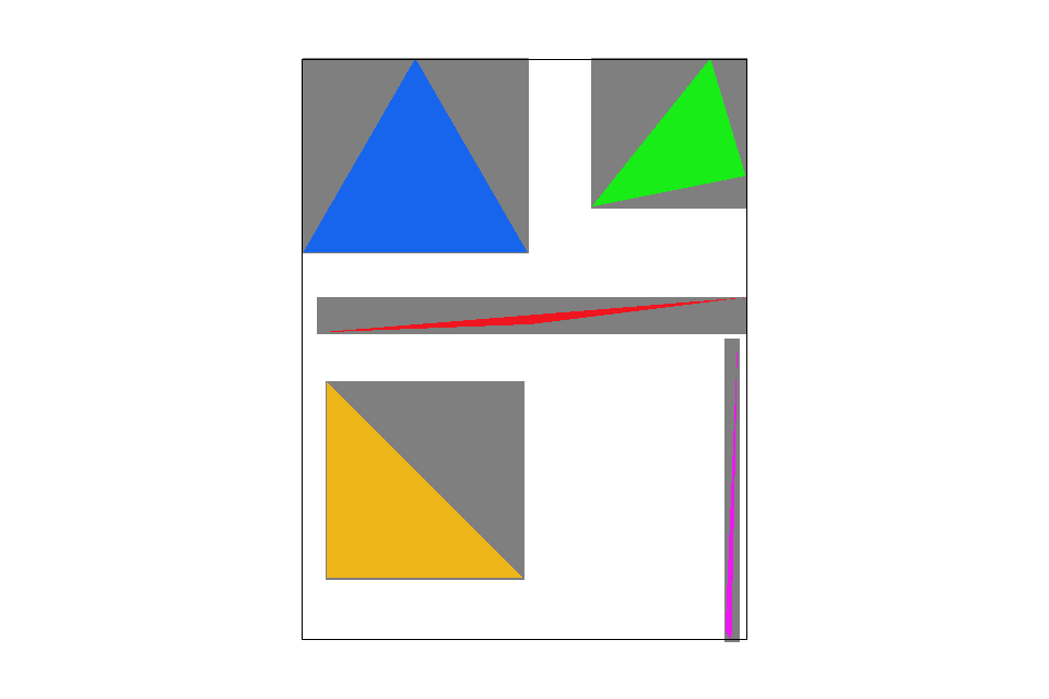
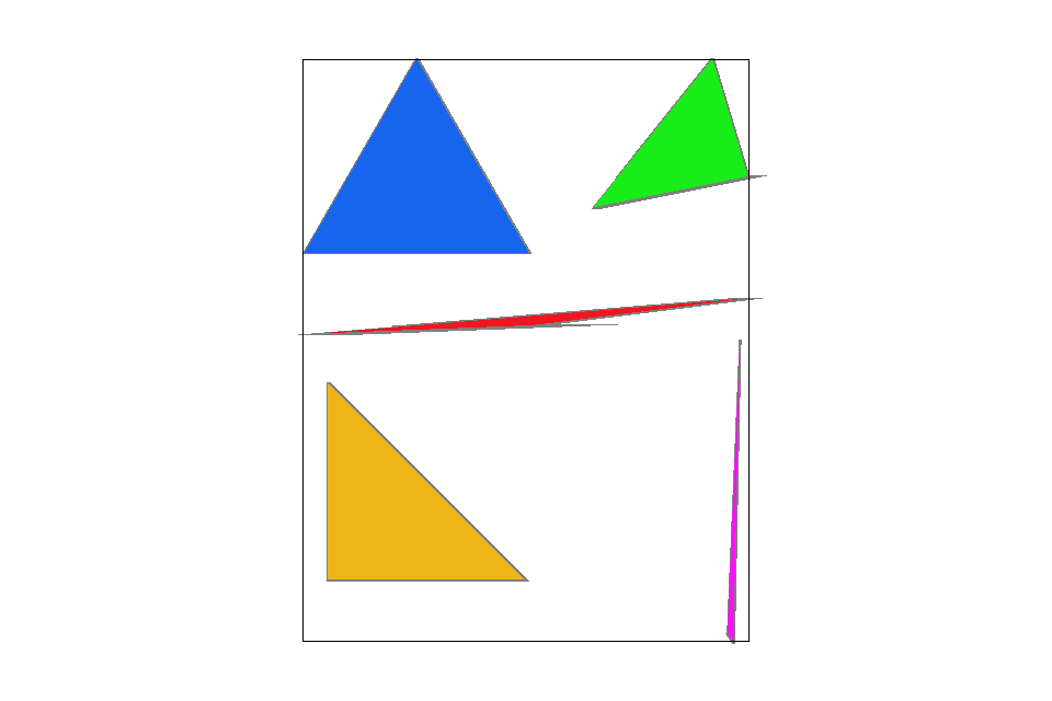
The area of pixels sampled (in gray) before/after implementing an optimized scanning approach.
One notable issue comes in with triangles with flatter slopes. For example, scanning the bottom half of the red triangle could require more padding along the sides to prevent pixels from missing due to numerical imprecision. After implementing this new approach to scanning, there is a performance increase of more than $35\%$ from local tests conducted.
Performance comparison with basic/test3.svg and basic/test4.svg, tested on MacBook Pro (Retina, 13-inch, Early 2013) with Apple LED Cinema Display, 24-inch (1920 x 1200).
In this project implementation, the scanning methods can be toggled with key C.
Part 2: Antialiasing triangles
In addition to sampling one point per-pixel, I implemented a basic supersampling scheme to begin with by uniformly increasing the sampling points per pixel. From the previous section, the value for a pixel $(x, y)^T$ can be sampled at $(x + 0.5, y + 0.5)^T$. Now, to support supersampling, the value for a pixel may be calculated as an average of subpixel values. And similar to the previous section, every subpixel is offset by $0.5$ in its area.
$$V_\text{sub}(x, y) = \text{value sampled at } (x + \frac{0.5}{\text{horizontal subpixels}}, y + \frac{0.5}{\text{vertical subpixels}})^T$$
Three-up comparison of basic/test4.svg at sampling rates 1 (top left), 4 (top right) and 16 (bottom).
Alternative sampling schemes (extra credit)
I experimented a little with a more randomized sampling scheme, where each sampling point is randomly placed within the subpixel. However, later I realized this probably will be a better approach for ray-tracing rather than for triangle rasterization: Since for a same subpixel the sampling point is randomized for every triangle, there could be times when randomized points in a subpixel lands on neither side of the triangle. This may produce the result as shown below. A good news is that the white line is partially removed because the sampling points are no longer aligned at the center of subpixels.
Comparison between sampling at pixel center and at random positions within the pixel.
To address the overwhelming randomness of the points being sampled per subpixel, I imagined using a hashing function to land sampling points, so for every subpixel there will be a constant lookup for an offset from the top left corner of the subpixel. And this renders a smoother but more dithered-looking image.
Comparison between sampling at pixel center and at consistent pseudo-random positions within the pixel.
Increasing the supersampling rate could produce fairly well result. Below are renderings of SVGs under the hardcore/ directory at a rate of 16.
Comparison of renderings of hardcore/01_degenerate_square1.svg by sampling at subpixel centers and at consistent pseudo-random subpixel locations.
There is little visual difference from supersampling between the two methods.
Comparison of renderings of hardcore/02_degenerate_square2.svg by sampling at subpixel centers and at consistent pseudo-random subpixel locations.
The example above has discrepancy at places along the center line; the new method has a more smudged effect. Using this method, there should only be a slight overhead to the existing sampling approach from the hashing function. In this project implementation, the sampling methods can be toggled with key A.
Part 3: Transforms
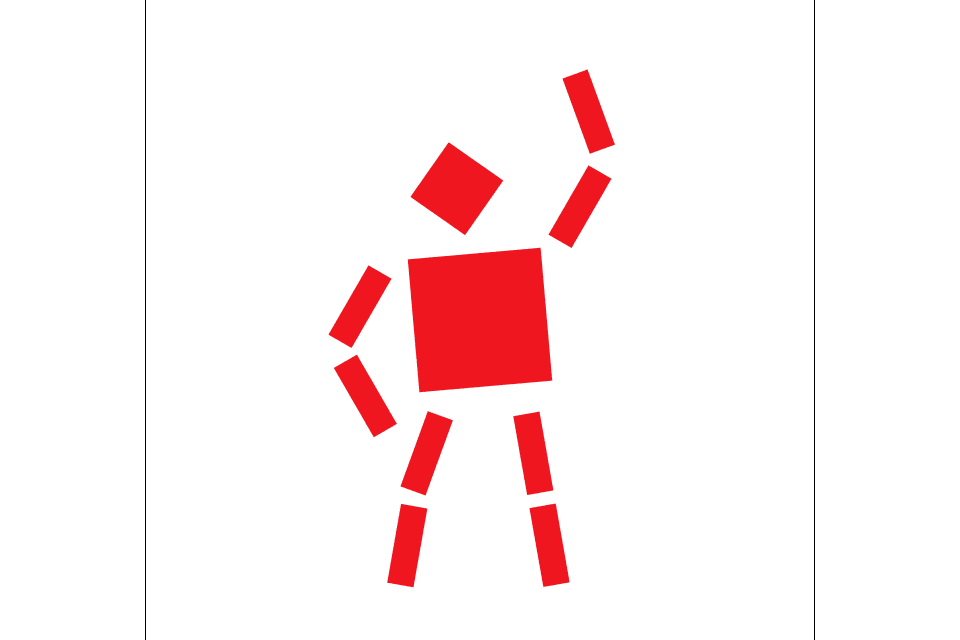
For this part, I planned to pose the robot as stretching. However, after tweaking the parameters, I landed on its waving hand to the viewer.
Robot waving hand, rendered with a supersampling rate of 16 and the hashing sampling approach mentioned above.
Introducing rotation at view center & better view moving (extra credit)
In addition to enabling transforms of geometric shapes, I added to the viewer an additional pair of controls to rotate the view port, Q to rotate CCW and E to rotate CW. In order to implement this feature, I tweaked the svg_to_ndc matrix that maps coordinates in SVG to normalized device coordinates. Initially, the matrix is defined as follows, given $x$, $y$ and $span$.
Since we are operating on homogeneous coordinates, the above matrix could be rewritten by scaling up the $w$ coordinate, rather than scaling down the $x$ and $y$ coordinates individually. Originally I made a mistake by scaling $x$, $y$ and $w$ coordinates all together, which ended up producing no effect on the target vector.
To explain each of the step in the transformation (from right to left), the viewing center on the SVG is first aligned to the origin, then shifted $span$ units in each direction ($x$ and $y$), and finally scaled down by $2 span$ to have the view area containe within $[0, 1]$ in each direction.
To enable rotation around the center of focus $(x, y)^T$, I inserted an additional matrix between the first and the second transformation, resulting in the following configuration. Note that at a viewing angle of $\theta$ radians CCW, we need to rotate the SVG the opposite amount (here $\theta$ radians CW).
The calculation above should be able to power void DrawRend::set_view(float x, float y, float span, float deg). However, void DrawRend::move_view(float dx, float dy, float zoom, float ddeg) needs to be able to read off the existing view properties from $M_{\text{svg} \to \text{ndc}}$. The current view angle $\theta$ could be easily reconstructed from $\cos(\theta)$ and $\sin(\theta)$ at the top left of the matrix. The current $span$ could be calculated by dividing the bottom right entry of the matrix by $2$. To find the current viewing center $(x, y)^T$, we can solve the following equation.
Then $(x, y)^T$ can be successfully recovered. With that, we are able to rotate around the viewing center.
Image sequence (in video) of rotating CCW around a star shape that's not at the center of the graph.
In addition to modifying the two methods mentioned above, I adjusted void DrawRend::cursor_event(float x, float y) to better convert from screen space to SVG coordinates, so it handles correct translations at different orientations and zoom levels utilizing the inverse of svg_to_ndc and ndc_to_screen matrices. Previously, moving mouse over a same distance on screen could result in mismatching translation of SVG. It's better to feel this enhancement in action by interacting with the viewer.
Section II: Sampling
Part 4: Barycentric coordinates
Barycentric coordinates allow us to describe the position of a point in relation to the vertices of a triangle. Suppose we take the vertices of a triangle, $\{\vec{a}, \vec{b}, \vec{c}\}$, we can decompose a point $\vec{p}$ into a linear combination of the three, allowing an easy linear interpolation of vertex attributes. To find the barycentric coordinates of a point, we can solve the following equation:
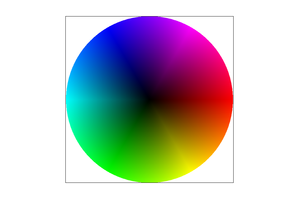
The last row is derived from the constraint $\alpha + \beta + \gamma = 1$. Below is an interactive example showing the barycentric coordinates of the mouse pointer position to the triangle, and an linear interpolation of colors where each of the vertex holds a primary color.
A
B
C
Interactive demo of barycentric coordinates with WebGL.
A rendering of basic/test7.svg with the default viewing parameters is shown below.
Part 5: Pixel sampling for texture mapping
Pixel sampling is a method to retrieve the color for a screen pixel, provided a texture image and the texture coordinates corresponding the pixel. Nearest sampling and bilinear sampling are two approaches mentioned in class to color a pixel with a texture map.
Nearest neighbor
Each vertex carries its UV coordinates (texture coordinates) that ranges from $0$ to $1$ in both directions. And we can use that piece of data, alongside the vertex positions, to interpolate the UV coordinates at each of the pixel over the triangle $(u, v)^T$. Suppose the texture has a dimension of w by h pixels. We can find the location that the UV coordinates land on the texture image $(u * w, v * h)^T$. Since the textural position may not be a full number, we can use nearest sampling to choose its closest neighboring pixel $(\lfloor u * w + 0.5 \rfloor, \lfloor v * h + 0.5 \rfloor)^T$ and get its value.
Bilinear
Similar to nearest sampling, rather than choosing the nearest neighbor, we choose all 4 neighboring vertices $\{(\lfloor u * w \rfloor, \lfloor v * h \rfloor)^T, (\lceil u * w \rceil, \lfloor v * h \rfloor)^T, (\lfloor u * w \rfloor, \lceil v * h \rceil)^T, (\lceil u * w \rceil, \lceil v * h \rceil)^T\}$ and interpolate their colors.
To linearly interpolate between two values, we can define $lerp(x, a, b) = (1 - x) * a + x * b$, where $x$ ranges between $0$ and $1$. With that, we can find the pixel color by interpolating the values of the top two pixels $\{(\lfloor u * w \rfloor, \lfloor v * h \rfloor)^T, (\lceil u * w \rceil, \lfloor v * h \rfloor)^T\}$ and of the bottom two pixels $\{(\lfloor u * w \rfloor, \lceil v * h \rceil)^T, (\lceil u * w \rceil, \lceil v * h \rceil)^T\}$ with $x = u * w - \lfloor u * w \rfloor$. Finally we can interpolate the intermediate values from the top and bottom edges with $x = v * h - \lfloor v * h \rfloor$.
Comparison
The differences could be significant between nearest neighbor and bilinear methods.
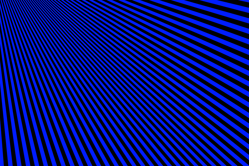
Nearest neighbor with a sampling rate of 1.Bilinear with a sampling rate of 1.
Nearest neighbor with a sampling rate of 16.Bilinear with a sampling rate of 16.
Since the texture image is sampled at a low sampling frequency in comparison to the dimension of the texture image, high contrast changes in pixel colors are possible subjects to aliasing. We can either bring up the sampling frequency (sampling with bilinear, shown with image on the top right) or reduce the overall frequency of the image being sampled (sampling at a rate of 16, shown with image on the bottom left). In comparison to nearest neighbor pixel sampling, both methods present possibilities to slightly reduce the aliasing problem. In the image shown, bilinear sampling at an initial sampling rate still shows some jaggies along the lines. The visual difference goes away slightly when we oversample the graph at a higher cost. Between nearest neighbor and bilinear sampling, supersampling at a rate of 16 does not present much visual difference.
Part 6: Level sampling with mipmaps for texture mapping
Since a texture at a high resolution could result in aliasing problems on small screen areas, mipmaps is a concept to minify textures as a set of smaller-sized texture maps to alleviate the high frequency signals. We use level sampling to choose an appropriate mipmap level for pixel sampling.
Zero level
With zero level sampling, we use the texture image as it is when sampling pixel colors.
Nearest level
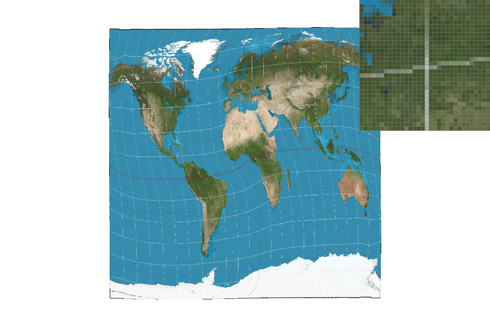
Similar to the concept of nearest neighbor pixel sampling, we would choose a mipmap level that fits the viewing box for pixel sampling. Suppose we have prepared a series of mipmaps, given a point on the framebuffer, we can find its corresponding texture coordinates on the texture map and also its footpring over the zero level texture image. For example, for a point at $(x, y)^T$, we can find its barycentric coordinates $(\alpha, \beta, \gamma)^T$ and interpolate its texture coordinates $(u, v)^T$ over the zero level image (not in an unit square). We can also estimate the size of its footprint by first finding the barycentric coordinates for $(x + 1, y)^T$ and $(x, y + 1)^T$ and then interpolating each UV coordinates, $(u_{dx}, v_{dx})^T$ and $(u_{dy}, v_{dy})^T$. The maximum coverage can be calculated as $l = \max(\sqrt{(u_{dx} - u)^2 + (v_{dx} - v)^2}, \sqrt{(u_{dy} - u)^2 + (v_{dy} - v)^2})$. Afterwards, we can choose a mipmap level $d = log_2{l}$; as an example, for a pixel with a footprint of 2 pixels (in texture coordinates), we will choose mipmap level one.
Comparison
Zero level and nearest neighbor pixel sampling.Zero level and bilinear pixel sampling.
Nearest level and nearest neighbor pixel sampling.Nearest level and bilinear pixel sampling.
Zero level is a clear winner in terms of memory usage since only a copy of the texture at its original dimensions is loaded to the memory. Nearest level sampling instead requires a series of levels of mipmaps before sampling. Typically image of a level up is one fourth of the size of the previous level; in total we will need about $\frac{1}{4} + \frac{1}{4}^2 + \frac{1}{4}^3 + \dots = \frac{1}{3}$ more space than storing a zero level texture map, not counting in the memory overhead.
Speed-wise, there is little extra constant computation per texture sampling to compute the mipmap level, making nearest level sampling a slightly slower option. Despite the memory and processing overhead, nearest level sampling presents a more decent rendering of the texture, avoiding jaggies from aliasing.
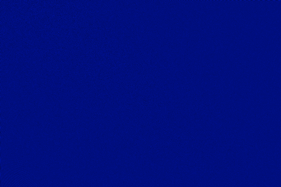
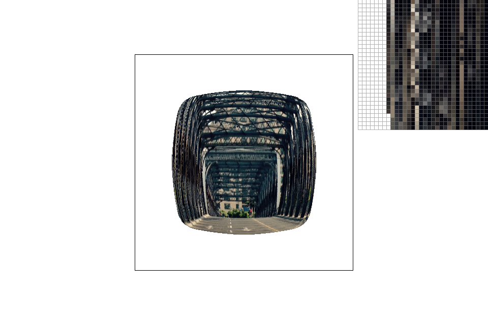
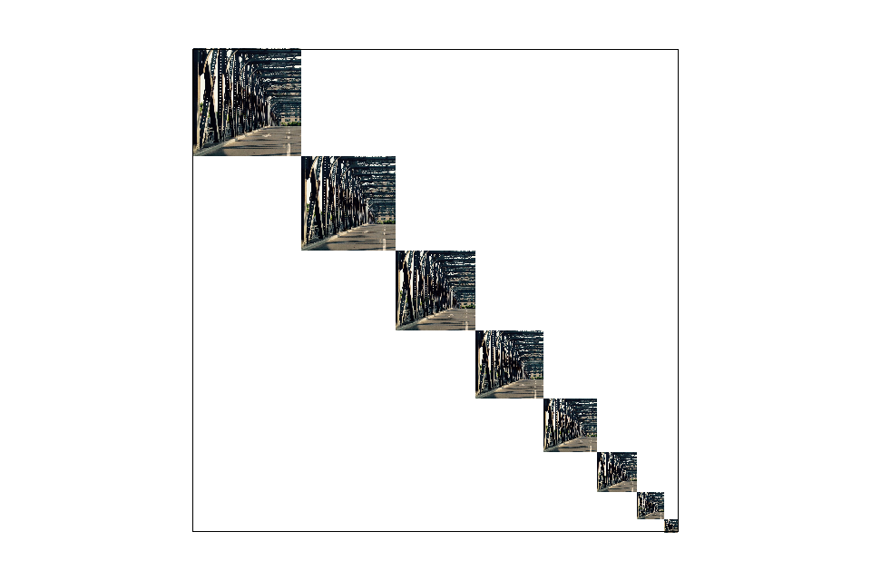
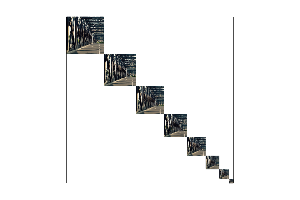
The two approaches present visual differences especially when a large texture is mapped to a small area for painting. Below is an example of this case.
Comparing zero level and nearest level sampling with nearest neighbor pixel sampling, squares' dimensions ranging from 80 by 80 to 10 by 10 pixels.
As showed in the image, the aliasing problem is greatly reduced with nearest level sampling.
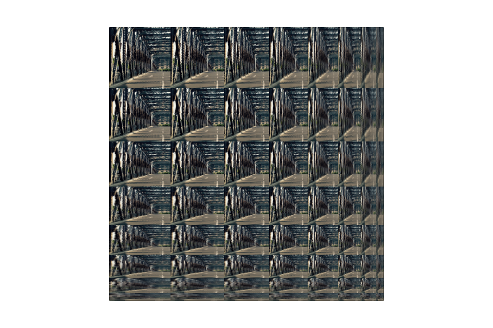
Anisotropic filtering (extra credit)
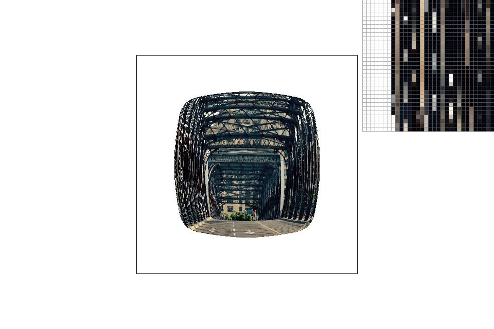
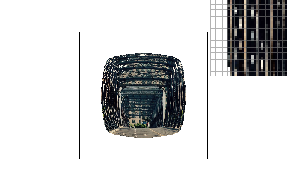
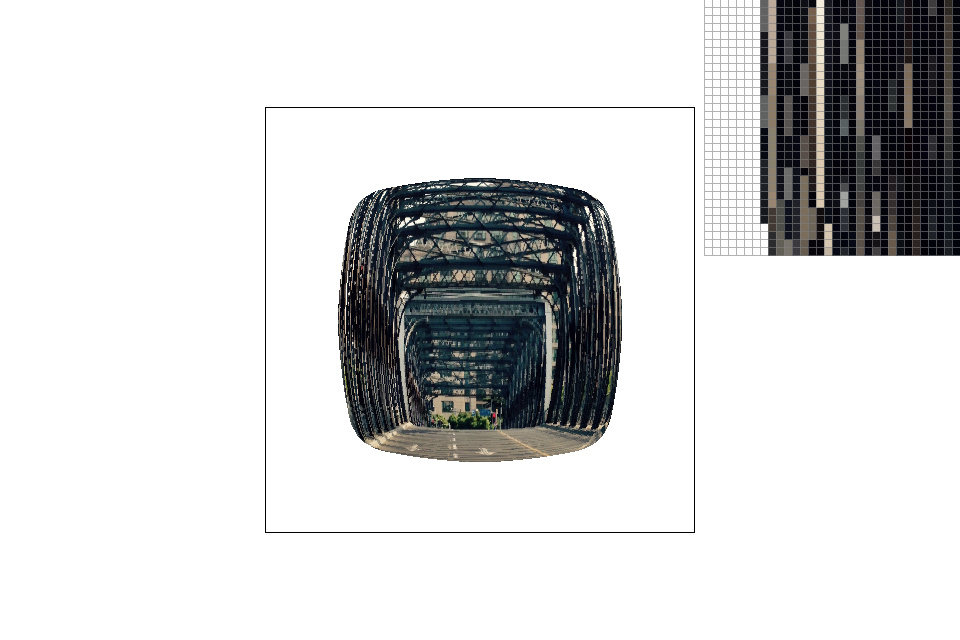
In addition to the above sampling schemes mentioned and trilinear sampling, I implemented anisotropic filtering. Below is an comparison with the trilinear sampling results. Visually speaking, anisotropic sampling produces a more accurate rendition of the texture image when viewed through differently sized windows.
Comparison of trilinear sampling results with anisotropic filtering enhancement at initial sampling rate.
Section III: Art Competition
Part 7: Draw something interesting!
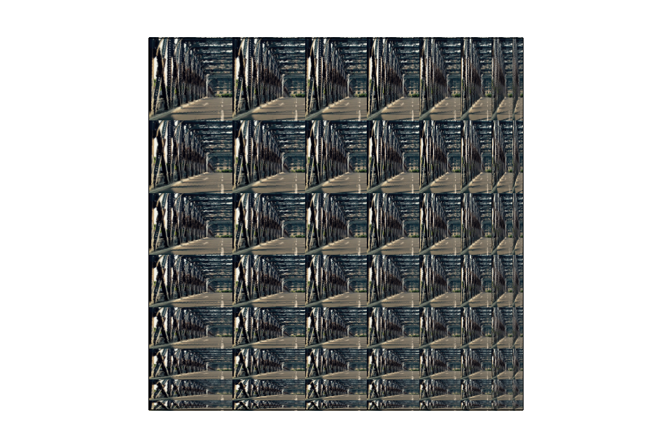
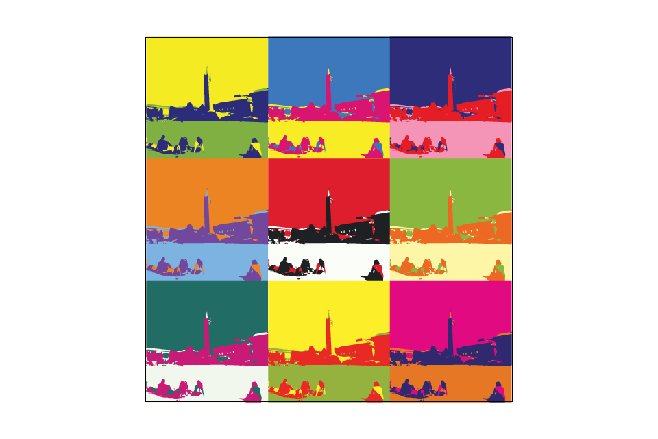
Memorial Glade & Campanile in pop art. How I did it: A couple of hours of manual image polygonization.